


A deep neural community might be understood as a geometrical system, the place every layer reshapes the enter house to type more and more complicated resolution boundaries. For this to work successfully, layers should protect significant spatial data — significantly how far an information level lies from these boundaries — since this distance allows deeper layers to construct wealthy, non-linear representations.
Sigmoid disrupts this course of by compressing all inputs right into a slim vary between 0 and 1. As values transfer away from resolution boundaries, they turn out to be indistinguishable, inflicting a lack of geometric context throughout layers. This results in weaker representations and limits the effectiveness of depth.
ReLU, however, preserves magnitude for optimistic inputs, permitting distance data to move by means of the community. This allows deeper fashions to stay expressive with out requiring extreme width or compute.
On this article, we deal with this forward-pass habits — analyzing how Sigmoid and ReLU differ in sign propagation and illustration geometry utilizing a two-moons experiment, and what meaning for inference effectivity and scalability.


Organising the dependencies
import numpy as np
import matplotlib.pyplot as plt
import matplotlib.gridspec as gridspec
from matplotlib.colours import ListedColormap
from sklearn.datasets import make_moons
from sklearn.preprocessing import StandardScaler
from sklearn.model_selection import train_test_split
plt.rcParams.replace({
"font.family": "monospace",
"axes.spines.top": False,
"axes.spines.right": False,
"figure.facecolor": "white",
"axes.facecolor": "#f7f7f7",
"axes.grid": True,
"grid.color": "#e0e0e0",
"grid.linewidth": 0.6,
})
T = {
"bg": "white",
"panel": "#f7f7f7",
"sig": "#e05c5c",
"relu": "#3a7bd5",
"c0": "#f4a261",
"c1": "#2a9d8f",
"text": "#1a1a1a",
"muted": "#666666",
}Creating the dataset
To check the impact of activation capabilities in a managed setting, we first generate an artificial dataset utilizing scikit-learn’s make_moons. This creates a non-linear, two-class downside the place easy linear boundaries fail, making it perfect for testing how effectively neural networks be taught complicated resolution surfaces.
We add a small quantity of noise to make the duty extra sensible, then standardize the options utilizing StandardScaler so each dimensions are on the identical scale — guaranteeing steady coaching. The dataset is then break up into coaching and take a look at units to judge generalization.
Lastly, we visualize the info distribution. This plot serves because the baseline geometry that each Sigmoid and ReLU networks will try and mannequin, permitting us to later examine how every activation perform transforms this house throughout layers.
X, y = make_moons(n_samples=400, noise=0.18, random_state=42)
X = StandardScaler().fit_transform(X)
X_train, X_test, y_train, y_test = train_test_split(
    X, y, test_size=0.25, random_state=42
)

fig, ax = plt.subplots(figsize=(7, 5))
fig.patch.set_facecolor(T["bg"])
ax.set_facecolor(T["panel"])
ax.scatter(X[y == 0, 0], X[y == 0, 1], c=T["c0"], s=40,
           edgecolors="white", linewidths=0.5, label="Class 0", alpha=0.9)
ax.scatter(X[y == 1, 0], X[y == 1, 1], c=T["c1"], s=40,
           edgecolors="white", linewidths=0.5, label="Class 1", alpha=0.9)
ax.set_title("make_moons -- our dataset", coloration=T["text"], fontsize=13)
ax.set_xlabel("x₁", coloration=T["muted"]); ax.set_ylabel("x₂", coloration=T["muted"])
ax.tick_params(colours=T["muted"]); ax.legend(fontsize=10)
plt.tight_layout()
plt.savefig("moons_dataset.png", dpi=140, bbox_inches="tight")
plt.present()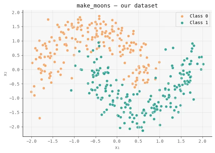
Creating the Community
Subsequent, we implement a small, managed neural community to isolate the impact of activation capabilities. The purpose right here is to not construct a extremely optimized mannequin, however to create a clear experimental setup the place Sigmoid and ReLU might be in contrast underneath an identical situations.
We outline each activation capabilities (Sigmoid and ReLU) together with their derivatives, and use binary cross-entropy because the loss since this can be a binary classification activity. The TwoLayerNet class represents a easy 3-layer feedforward community (2 hidden layers + output), the place the one configurable part is the activation perform.
A key element is the initialization technique: we use He initialization for ReLU and Xavier initialization for Sigmoid, guaranteeing that every community begins in a good and steady regime primarily based on its activation dynamics.
The ahead go computes activations layer by layer, whereas the backward go performs normal gradient descent updates. Importantly, we additionally embody diagnostic strategies like get_hidden and get_z_trace, which permit us to examine how indicators evolve throughout layers — that is essential for analyzing how a lot geometric data is preserved or misplaced.
By preserving structure, knowledge, and coaching setup fixed, this implementation ensures that any distinction in efficiency or inner representations might be straight attributed to the activation perform itself — setting the stage for a transparent comparability of their influence on sign propagation and expressiveness.
def sigmoid(z):      return 1 / (1 + np.exp(-np.clip(z, -500, 500)))
def sigmoid_d(a):    return a * (1 - a)
def relu(z):         return np.most(0, z)
def relu_d(z):       return (z > 0).astype(float)
def bce(y, yhat):    return -np.imply(y * np.log(yhat + 1e-9) + (1 - y) * np.log(1 - yhat + 1e-9))

class TwoLayerNet:
    def __init__(self, activation="relu", seed=0):
        np.random.seed(seed)
        self.act_name = activation
        self.act  = relu    if activation == "relu" else sigmoid
        self.dact = relu_d  if activation == "relu" else sigmoid_d

        # He init for ReLU, Xavier for Sigmoid
        scale = lambda fan_in: np.sqrt(2 / fan_in) if activation == "relu" else np.sqrt(1 / fan_in)
        self.W1 = np.random.randn(2, 8)  * scale(2)
        self.b1 = np.zeros((1, 8))
        self.W2 = np.random.randn(8, 8)  * scale(8)
        self.b2 = np.zeros((1, 8))
        self.W3 = np.random.randn(8, 1)  * scale(8)
        self.b3 = np.zeros((1, 1))
        self.loss_history = []

    def ahead(self, X, retailer=False):
        z1 = X  @ self.W1 + self.b1;  a1 = self.act(z1)
        z2 = a1 @ self.W2 + self.b2;  a2 = self.act(z2)
        z3 = a2 @ self.W3 + self.b3;  out = sigmoid(z3)
        if retailer:
            self._cache = (X, z1, a1, z2, a2, z3, out)
        return out

    def backward(self, lr=0.05):
        X, z1, a1, z2, a2, z3, out = self._cache
        n = X.form[0]

        dout = (out - self.y_cache) / n
        dW3 = a2.T @ dout;  db3 = dout.sum(axis=0, keepdims=True)
        da2 = dout @ self.W3.T
        dz2 = da2 * (self.dact(z2) if self.act_name == "relu" else self.dact(a2))
        dW2 = a1.T @ dz2;  db2 = dz2.sum(axis=0, keepdims=True)
        da1 = dz2 @ self.W2.T
        dz1 = da1 * (self.dact(z1) if self.act_name == "relu" else self.dact(a1))
        dW1 = X.T  @ dz1;  db1 = dz1.sum(axis=0, keepdims=True)

        for p, g in [(self.W3,dW3),(self.b3,db3),(self.W2,dW2),
                     (self.b2,db2),(self.W1,dW1),(self.b1,db1)]:
            p -= lr * g

    def train_step(self, X, y, lr=0.05):
        self.y_cache = y.reshape(-1, 1)
        out = self.ahead(X, retailer=True)
        loss = bce(self.y_cache, out)
        self.backward(lr)
        return loss

    def get_hidden(self, X, layer=1):
        """Return post-activation values for layer 1 or 2."""
        z1 = X @ self.W1 + self.b1;  a1 = self.act(z1)
        if layer == 1: return a1
        z2 = a1 @ self.W2 + self.b2; return self.act(z2)

    def get_z_trace(self, x_single):
        """Return pre-activation magnitudes per layer for ONE sample."""
        z1 = x_single @ self.W1 + self.b1
        a1 = self.act(z1)
        z2 = a1 @ self.W2 + self.b2
        a2 = self.act(z2)
        z3 = a2 @ self.W3 + self.b3
        return [np.abs(z1).mean(), np.abs(a1).mean(),
                np.abs(z2).mean(), np.abs(a2).mean(),
                np.abs(z3).mean()]
Coaching the Networks
Now we prepare each networks underneath an identical situations to make sure a good comparability. We initialize two fashions — one utilizing Sigmoid and the opposite utilizing ReLU — with the identical random seed so they begin from equal weight configurations.
The coaching loop runs for 800 epochs utilizing mini-batch gradient descent. In every epoch, we shuffle the coaching knowledge, break up it into batches, and replace each networks in parallel. This setup ensures that the one variable altering between the 2 runs is the activation perform.
We additionally monitor the loss after each epoch and log it at common intervals. This permits us to watch how every community evolves over time — not simply when it comes to convergence pace, however whether or not it continues enhancing or plateaus.
This step is vital as a result of it establishes the primary sign of divergence: if each fashions begin identically however behave in another way throughout coaching, that distinction should come from how every activation perform propagates and preserves data by means of the community.
EPOCHS = 800
LR     = 0.05
BATCH  = 64

net_sig  = TwoLayerNet("sigmoid", seed=42)
net_relu = TwoLayerNet("relu",    seed=42)

for epoch in vary(EPOCHS):
    idx = np.random.permutation(len(X_train))
    for internet in [net_sig, net_relu]:
        epoch_loss = []
        for i in vary(0, len(idx), BATCH):
            b = idx[i:i+BATCH]
            loss = internet.train_step(X_train[b], y_train[b], LR)
            epoch_loss.append(loss)
        internet.loss_history.append(np.imply(epoch_loss))

    if (epoch + 1) % 200 == 0:
        ls = net_sig.loss_history[-1]
        lr = net_relu.loss_history[-1]
        print(f"  Epoch {epoch+1:4d} | Sigmoid loss: {ls:.4f} | ReLU loss: {lr:.4f}")

print("n✅ Training complete.")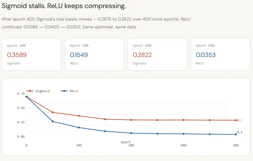
Coaching Loss Curve
The loss curves make the divergence between Sigmoid and ReLU very clear. Each networks begin from the identical initialization and are skilled underneath an identical situations, but their studying trajectories rapidly separate. Sigmoid improves initially however plateaus round ~0.28 by epoch 400, displaying virtually no progress afterward — an indication that the community has exhausted the helpful sign it may extract.
ReLU, in distinction, continues to steadily cut back loss all through coaching, dropping from ~0.15 to ~0.03 by epoch 800. This isn’t simply quicker convergence; it displays a deeper challenge: Sigmoid’s compression is limiting the move of significant data, inflicting the mannequin to stall, whereas ReLU preserves that sign, permitting the community to maintain refining its resolution boundary.
fig, ax = plt.subplots(figsize=(10, 5))
fig.patch.set_facecolor(T["bg"])
ax.set_facecolor(T["panel"])

ax.plot(net_sig.loss_history,  coloration=T["sig"],  lw=2.5, label="Sigmoid")
ax.plot(net_relu.loss_history, coloration=T["relu"], lw=2.5, label="ReLU")

ax.set_xlabel("Epoch", coloration=T["muted"])
ax.set_ylabel("Binary Cross-Entropy Loss", coloration=T["muted"])
ax.set_title("Training Loss -- same architecture, same init, same LRnonly the activation differs",
             coloration=T["text"], fontsize=12)
ax.legend(fontsize=11)
ax.tick_params(colours=T["muted"])

# Annotate remaining losses
for internet, coloration, va in [(net_sig, T["sig"], "bottom"), (net_relu, T["relu"], "top")]:
    remaining = internet.loss_history[-1]
    ax.annotate(f"  final: {final:.4f}", xy=(EPOCHS-1, remaining),
                coloration=coloration, fontsize=9, va=va)

plt.tight_layout()
plt.savefig("loss_curves.png", dpi=140, bbox_inches="tight")
plt.present()
Choice Boundary Plots
The choice boundary visualization makes the distinction much more tangible. The Sigmoid community learns an almost linear boundary, failing to seize the curved construction of the two-moons dataset, which ends up in decrease accuracy (~79%). This can be a direct consequence of its compressed inner representations — the community merely doesn’t have sufficient geometric sign to assemble a posh boundary.
In distinction, the ReLU community learns a extremely non-linear, well-adapted boundary that intently follows the info distribution, reaching a lot larger accuracy (~96%). As a result of ReLU preserves magnitude throughout layers, it allows the community to progressively bend and refine the choice floor, turning depth into precise expressive energy moderately than wasted capability.
def plot_boundary(ax, internet, X, y, title, coloration):
    h = 0.025
    x_min, x_max = X[:, 0].min() - 0.5, X[:, 0].max() + 0.5
    y_min, y_max = X[:, 1].min() - 0.5, X[:, 1].max() + 0.5
    xx, yy = np.meshgrid(np.arange(x_min, x_max, h),
                         np.arange(y_min, y_max, h))
    grid = np.c_[xx.ravel(), yy.ravel()]
    Z = internet.ahead(grid).reshape(xx.form)

    # Smooth shading
    cmap_bg = ListedColormap(["#fde8c8", "#c8ece9"])
    ax.contourf(xx, yy, Z, ranges=50, cmap=cmap_bg, alpha=0.85)
    ax.contour(xx, yy, Z, ranges=[0.5], colours=[color], linewidths=2)

    ax.scatter(X[y==0, 0], X[y==0, 1], c=T["c0"], s=35,
               edgecolors="white", linewidths=0.4, alpha=0.9)
    ax.scatter(X[y==1, 0], X[y==1, 1], c=T["c1"], s=35,
               edgecolors="white", linewidths=0.4, alpha=0.9)

    acc = ((internet.ahead(X) >= 0.5).ravel() == y).imply()
    ax.set_title(f"{title}nTest acc: {acc:.1%}", coloration=coloration, fontsize=12)
    ax.set_xlabel("x₁", coloration=T["muted"]); ax.set_ylabel("x₂", coloration=T["muted"])
    ax.tick_params(colours=T["muted"])

fig, axes = plt.subplots(1, 2, figsize=(13, 5.5))
fig.patch.set_facecolor(T["bg"])
fig.suptitle("Decision Boundaries learned on make_moons",
             fontsize=13, coloration=T["text"])

plot_boundary(axes[0], net_sig,  X_test, y_test, "Sigmoid", T["sig"])
plot_boundary(axes[1], net_relu, X_test, y_test, "ReLU",    T["relu"])

plt.tight_layout()
plt.savefig("decision_boundaries.png", dpi=140, bbox_inches="tight")
plt.present()
Layer-by-Layer Sign Hint
This chart tracks how the sign evolves throughout layers for some extent removed from the choice boundary — and it clearly exhibits the place Sigmoid fails. Each networks begin with comparable pre-activation magnitude on the first layer (~2.0), however Sigmoid instantly compresses it to ~0.3, whereas ReLU retains the next worth. As we transfer deeper, Sigmoid continues to squash the sign right into a slim band (0.5–0.6), successfully erasing significant variations. ReLU, however, preserves and amplifies magnitude, with the ultimate layer reaching values as excessive as 9–20.
This implies the output neuron within the ReLU community is making selections primarily based on a robust, well-separated sign, whereas the Sigmoid community is compelled to categorise utilizing a weak, compressed one. The important thing takeaway is that ReLU preserves distance from the choice boundary throughout layers, permitting that data to compound, whereas Sigmoid progressively destroys it.
far_class0 = X_train[y_train == 0][np.argmax(
    np.linalg.norm(X_train[y_train == 0] - [-1.2, -0.3], axis=1)
)]
far_class1 = X_train[y_train == 1][np.argmax(
    np.linalg.norm(X_train[y_train == 1] - [1.2, 0.3], axis=1)
)]

stage_labels = ["z₁ (pre)", "a₁ (post)", "z₂ (pre)", "a₂ (post)", "z₃ (out)"]
x_pos = np.arange(len(stage_labels))

fig, axes = plt.subplots(1, 2, figsize=(13, 5.5))
fig.patch.set_facecolor(T["bg"])
fig.suptitle("Layer-by-layer signal magnitude -- a point far from the boundary",
             fontsize=12, coloration=T["text"])

for ax, pattern, title in zip(
    axes,
    [far_class0, far_class1],
    ["Class 0 sample (deep in its moon)", "Class 1 sample (deep in its moon)"]
):
    ax.set_facecolor(T["panel"])
    sig_trace  = net_sig.get_z_trace(pattern.reshape(1, -1))
    relu_trace = net_relu.get_z_trace(pattern.reshape(1, -1))

    ax.plot(x_pos, sig_trace,  "o-", coloration=T["sig"],  lw=2.5, markersize=8, label="Sigmoid")
    ax.plot(x_pos, relu_trace, "s-", coloration=T["relu"], lw=2.5, markersize=8, label="ReLU")

    for i, (s, r) in enumerate(zip(sig_trace, relu_trace)):
        ax.textual content(i, s - 0.06, f"{s:.3f}", ha="center", fontsize=8, coloration=T["sig"])
        ax.textual content(i, r + 0.04, f"{r:.3f}", ha="center", fontsize=8, coloration=T["relu"])

    ax.set_xticks(x_pos); ax.set_xticklabels(stage_labels, coloration=T["muted"], fontsize=9)
    ax.set_ylabel("Mean |activation|", coloration=T["muted"])
    ax.set_title(title, coloration=T["text"], fontsize=11)
    ax.tick_params(colours=T["muted"]); ax.legend(fontsize=10)

plt.tight_layout()
plt.savefig("signal_trace.png", dpi=140, bbox_inches="tight")
plt.present()
Hidden Area Scatter
That is a very powerful visualization as a result of it straight exposes how every community makes use of (or fails to make use of) depth. Within the Sigmoid community (left), each courses collapse into a good, overlapping area — a diagonal smear the place factors are closely entangled. The usual deviation truly decreases from layer 1 (0.26) to layer 2 (0.19), which means the illustration is changing into much less expressive with depth. Every layer is compressing the sign additional, stripping away the spatial construction wanted to separate the courses.
ReLU exhibits the other habits. In layer 1, whereas some neurons are inactive (the “dead zone”), the lively ones already unfold throughout a wider vary (1.15 std), indicating preserved variation. By layer 2, this expands even additional (1.67 std), and the courses turn out to be clearly separable — one is pushed to excessive activation ranges whereas the opposite stays close to zero. At this level, the output layer’s job is trivial.
fig, axes = plt.subplots(2, 2, figsize=(13, 10))
fig.patch.set_facecolor(T["bg"])
fig.suptitle("Hidden-space representations on make_moons test set",
             fontsize=13, coloration=T["text"])

for col, (internet, coloration, title) in enumerate([
    (net_sig,  T["sig"],  "Sigmoid"),
    (net_relu, T["relu"], "ReLU"),
]):
    for row, layer in enumerate([1, 2]):
        ax = axes[row][col]
        ax.set_facecolor(T["panel"])
        H = internet.get_hidden(X_test, layer=layer)

        ax.scatter(H[y_test==0, 0], H[y_test==0, 1], c=T["c0"], s=40,
                   edgecolors="white", linewidths=0.4, alpha=0.85, label="Class 0")
        ax.scatter(H[y_test==1, 0], H[y_test==1, 1], c=T["c1"], s=40,
                   edgecolors="white", linewidths=0.4, alpha=0.85, label="Class 1")

        unfold = H.std()
        ax.textual content(0.04, 0.96, f"std: {spread:.4f}",
                rework=ax.transAxes, fontsize=9, va="top",
                coloration=T["text"],
                bbox=dict(boxstyle="round,pad=0.3", fc="white", ec=coloration, alpha=0.85))

        ax.set_title(f"{name}  --  Layer {layer} hidden space",
                     coloration=coloration, fontsize=11)
        ax.set_xlabel(f"Unit 1", coloration=T["muted"])
        ax.set_ylabel(f"Unit 2", coloration=T["muted"])
        ax.tick_params(colours=T["muted"])
        if row == 0 and col == 0: ax.legend(fontsize=9)

plt.tight_layout()
plt.savefig("hidden_space.png", dpi=140, bbox_inches="tight")
plt.present()

Take a look at the Full Codes right here. Additionally, be at liberty to comply with us on Twitter and don’t overlook to affix our 120k+ ML SubReddit and Subscribe to our E-newsletter. Wait! are you on telegram? now you’ll be able to be part of us on telegram as effectively.
Have to associate with us for selling your GitHub Repo OR Hugging Face Web page OR Product Launch OR Webinar and many others.? Join with us

I’m a Civil Engineering Graduate (2022) from Jamia Millia Islamia, New Delhi, and I’ve a eager curiosity in Information Science, particularly Neural Networks and their utility in numerous areas.