



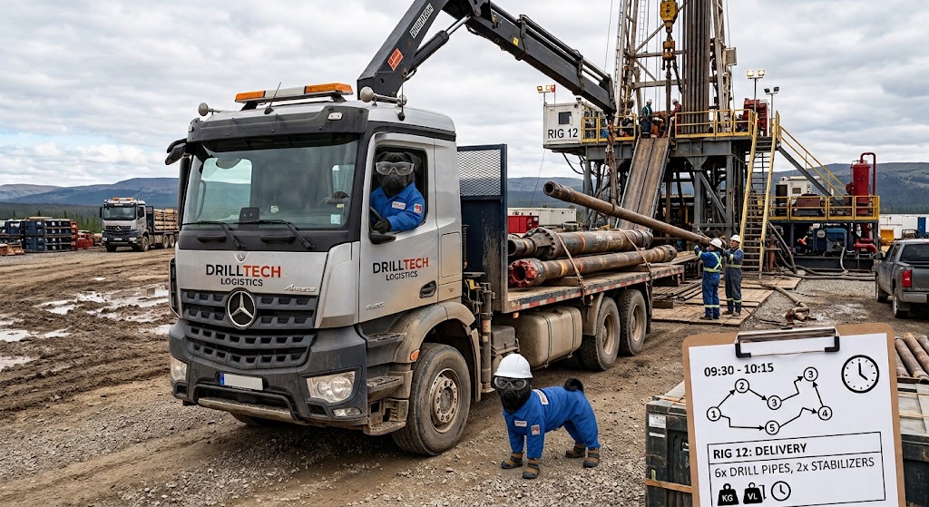
**From “Los Movimientos” to a Full Optimization Model: Solving Complex Vehicle Routing for Drill‑Crew Transport**
—
### Introduction
Few things in operations research can make an engineer’s stomach drop faster than the words *“Los Movimientos.”* In this article, I take you back to my time working in oil and gas logistics in eastern Venezuela, where every afternoon was spent coordinating dozens of truck movements under tight time windows, scarce shared fleet resources, and strict safety rules.
Today, with the benefit of operations research training, I show how those chaotic afternoons map directly to a well‑known combinatorial optimization problem: **the Capacitated Pickup and Delivery Vehicle Routing Problem with Time Windows (PDPTW)**.
By the end of this article, you will see how to:
– Formalize a real‑world dispatch problem as a PDPTW
– Build a mixed‑integer linear programming (MILP) model in Pyomo
– Solve it with the open‑source HiGHS optimizer
– Extract readable routes and visualize them
– Interpret results to answer practical questions such as whether more trucks are needed
The full walkthrough—including data, model, code, and plots—is implemented in a publicly available GitHub repository, but the concepts here apply to any pickup‑and‑delivery logistics challenge (e‑commerce, field service, medical transport, waste collection, etc.).
—
### The Problem: When Every Delivery Also Comes with a Pickup
Many logistics tasks involve **paired operations**: a vehicle must pick up an item and later deliver it. Examples include:
– Grocery delivery with reusable containers
– Furniture delivery with old‑appliance take‑back
– Oilfield service: picking up tools at a base and delivering them to a rig
In these settings, each *request* consists of:
1. **Pickup** (load increases)
2. **Delivery** (load decreases)
3. A **precedence constraint**: pickup must occur before delivery
4. A **single vehicle** must handle both operations
Additionally, real operations impose:
– **Time windows** for each pickup and delivery
– **Vehicle capacity limits**
– **Heterogeneous fleet** and compatibility requirements
– **Multiple start/end locations** (vehicles not always at the same depot)
– **Limited fleet size**, which can make some requests unserved
These characteristics define the **Capacitated Pickup and Delivery Vehicle Routing Problem with Time Windows (PDPTW)**—a notoriously difficult mixed‑integer programming problem.
—
### Modeling the PDPTW
#### Decision Variables
The model uses four main variables:
– **x[k,i,j]**: binary, equals 1 if vehicle *k* travels from node *i* to node *j*
– **z[r]**: binary, equals 1 if request *r* is left unserved (placed in a “request bank”)
– **S[k,i]**: service start time for vehicle *k* at node *i*
– **L[k,i]**: load of vehicle *k* after servicing node *i*
#### Objective Function
We minimize a weighted sum of:
1. Total distance traveled
2. Total vehicle operating time
3. A large penalty for each unserved request
This ensures the solver first tries to serve all requests, using distance and time only as tie‑breakers.
#### Key Constraints
In plain language:
1. **Request handling**: Each request is either served by one compatible vehicle or left unserved.
2. **Pickup–delivery pairing**: The same vehicle performs both pickup and delivery.
3. **Route continuity**: Every vehicle leaves its start and arrives at its end exactly once.
4. **Flow conservation**: If a vehicle arrives at a node, it must leave it.
5. **Time propagation**: Arrival + service + travel ≤ next service start (with “big‑M” penalties when an arc is unused).
6. **Precedence**: Pickup time ≤ delivery time for each request.
7. **Load propagation**: Load increases at pickups, decreases at deliveries.
8. **Capacity**: Load always stays between 0 and vehicle capacity.
9. **Vehicle terminals**: All vehicles start and end empty.
10. **Binary decisions**: Routing and request‑bank variables are 0 or 1.
Together, these constraints encode the exact “Los Movimientos” reality described in the opening paragraphs.
—
### A Small but Realistic Example
To keep things tractable, I built a toy instance with:
– 3 identical pickup trucks
– 10 personnel‑transport requests
– One operational base and five drilling rigs
– Time windows (including a hard no‑drive window after 8 p.m.)
– A capacity of 3 passengers per vehicle
Travel times and distances are symmetric and deterministic. Each request involves moving a group of workers, with pickup and delivery windows aligned with shift changes.
You can reproduce this example by downloading the JSON instance and running the Python code shown in the article, which:
– Loads the data
– Builds nodes, arcs, and “big‑M” values
– Constructs the full Pyomo model
– Solves with HiGHS (open‑source)
– Prints a driver‑friendly itinerary
—
### Results and Visualization
The solver produced three efficient routes:
– **PU_1**: Base → Rig A → Rig D → Rig B (Base)
– **PU_2**: Base → Rig C → Rig A → Rig B → Rig C → Rig A → Base
– **PU_3**: Base → Rig B → Rig E → Rig A → Base
Each route respects time windows, capacity, and precedence. The optimization also revealed that all ten requests were served—no extra truck was needed.
I visualized the routes on a 2D map, showing stop order, arrival times, and passenger counts, making it easy for dispatchers to understand and communicate the plan.
—
### Conclusions
This article shows that even the most stressful routing problems—like “Los Movimientos”—can be tamed with a formal optimization model. The PDPTW formulation captures real‑world complexity while remaining solvable with modern open‑source tools.
Key takeaways:
– A clear model is more valuable than ad‑hoc heuristics
– Optimization can tell you not only *how* to route, but also *whether your resources are sufficient*
– The best solution is not always the one that looks most “efficient” at first glance
– Models must be paired with good user interfaces to be usable in practice
As operations grow, exact MILP may become too slow, leading naturally to **large‑neighborhood search (LNS)** heuristics—a topic for a future article.
If you’ve faced similar routing or dispatching challenges, I’d love to hear how you approached them. Feel free to explore the full code and data in the accompanying repository and adapt the model to your own problems.
**Thanks for reading—and to my former teammates who inspired this journey.**
