



# Reconstructing Blood Flow with Physics-Informed Neural Networks: A PINN Approach for Stenosed Arteries
## Introduction
Blood flowing through arteries exerts a frictional force on vessel walls known as wall shear stress. This quantity plays a critical role in understanding where atherosclerotic plaque develops, yet it remains notoriously difficult to measure directly in clinical settings. A typical Doppler ultrasound examination provides velocity readings at only a handful of discrete points inside a vessel, leaving large gaps in our knowledge of the full flow field.
The central question is whether a neural network can take these sparse, noisy velocity measurements and combine them with the governing equations of fluid dynamics to reconstruct the entire flow field, including the wall shear stress at the vessel boundary.
Physics-informed neural networks offer a compelling answer. Unlike standard neural networks that learn purely from data, PINNs embed the physical laws governing a system directly into their training objective. This article demonstrates how a PINN built entirely in PyTorch can reconstruct the complete velocity and pressure fields of blood flow through a stenosed artery from just forty noisy velocity readings. The network simultaneously estimates the fluid viscosity as an unknown parameter and accurately captures the wall shear stress profile, matching results from conventional computational fluid dynamics simulations.
—
## Modeling the Artery Geometry and Flow Conditions
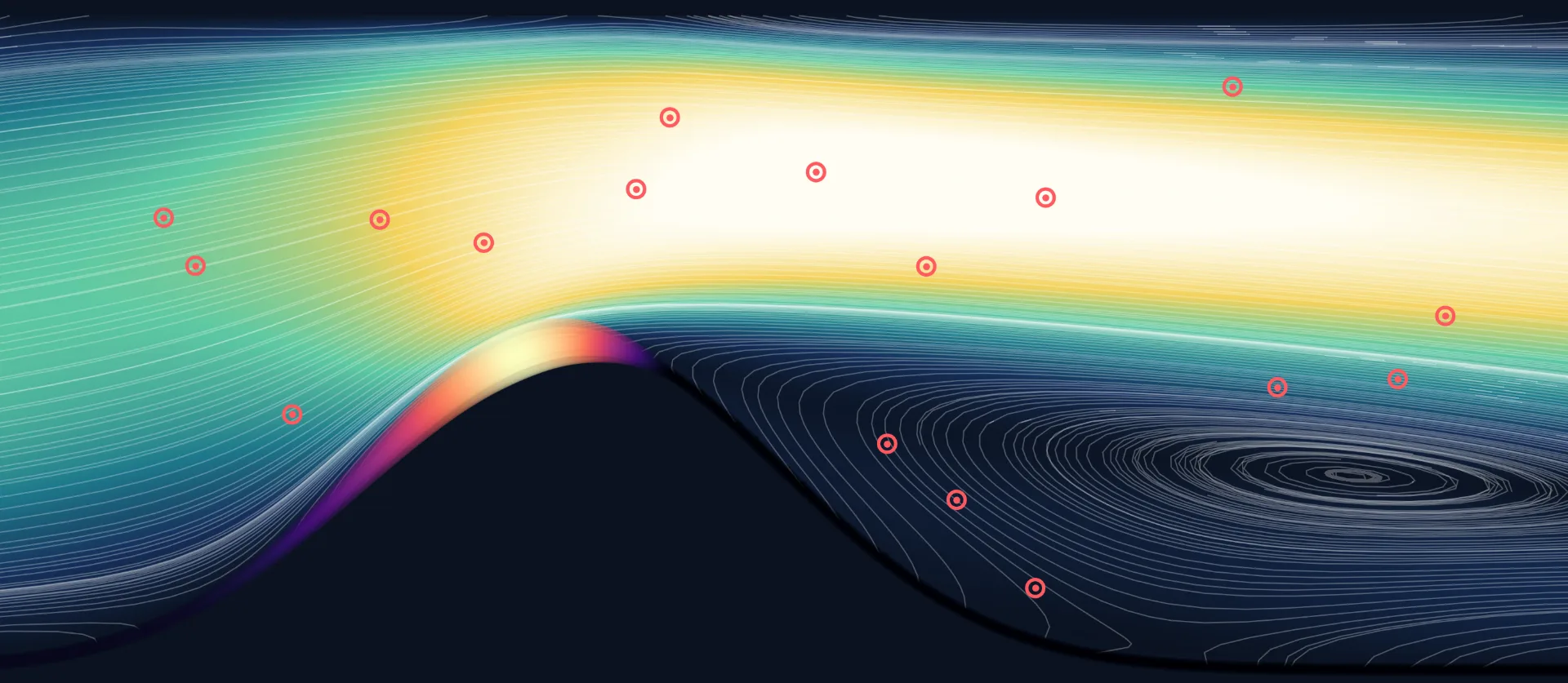
The study considers a two-dimensional channel representing a cross-section of an artery. The channel has a uniform height, and a smooth narrowing on the lower wall creates a fifty-percent stenosis—effectively blocking half of the opening. This geometry produces a flow pattern rich enough to test the capabilities of a neural network reconstruction, including regions of accelerated flow through the throat and separated, reversed flow downstream of the obstruction.
The flow is governed by the incompressible Navier-Stokes equations at a Reynolds number of two hundred, which places it in the low-to-moderate range typical of carotid artery flows. All quantities are normalized by the channel height and inlet velocity, which means the kinematic viscosity takes the value of 0.005 in these dimensionless units.
A key practical decision concerns the length of the computational domain. In a shorter domain, the region of reversed flow behind the stenosis fails to close before the outlet boundary, meaning the outlet condition influences the entire solution and distorts the reference data. Extending the channel to nine channel heights ensures the reversed flow region terminates naturally at approximately x equals 5.8, leaving a fully developed forward flow region toward the outlet where boundary assumptions no longer corrupt the physics.
The training data consists of forty velocity probes placed inside the fluid domain. Each probe provides a two-dimensional velocity vector corrupted by Gaussian noise at seven percent of the inlet velocity magnitude. Critically, no pressure measurements are available, and no probes sit directly on the wall. The sensors are distributed across four bands along the channel, with greater density near the throat of the stenosis and in the wake region where the flow physics are most complex.
—
## The Neural Network Architecture
The PINN is a standard multilayer perceptron with six hidden layers, each containing thirty-two units with hyperbolic tangent activation functions. The total parameter count is approximately 5,500 weights and biases. The choice of hyperbolic tangent over alternatives like ReLU is deliberate: the Navier-Stokes equations require second derivatives of the network output with respect to spatial coordinates, and the second derivative of a ReLU is zero almost everywhere, which would prevent meaningful gradient flow. The hyperbolic tangent function is smooth and infinitely differentiable, making it well-suited for physics-informed problems.
The network takes spatial coordinates (x, y) as input and produces three outputs: the streamwise velocity u, the wall-normal velocity v, and the pressure p. Input coordinates are rescaled to the range negative one to one internally, which helps with training stability while preserving the ability to compute derivatives with respect to the original physical coordinates through automatic differentiation.
—
## Implementing the Navier-Stokes Residual in PyTorch
The core of the PINN approach is computing how well the network’s output satisfies the Navier-Stokes equations at arbitrary points in the domain. This is accomplished through automatic differentiation, a built-in feature of PyTorch that computes exact derivatives through the computational graph.
The implementation computes first derivatives of velocity and pressure with respect to both spatial coordinates, then second derivatives of the velocity components. These are assembled into three residual equations:
– **Continuity**: the divergence of the velocity field, which must equal zero for incompressible flow.
– **Momentum in the streamwise direction**: balancing convective acceleration, pressure gradient, and viscous diffusion.
– **Momentum in the wall-normal direction**: the same balance for the transverse component.
A helper function computes gradients by calling `torch.autograd.grad` with `create_graph=True` and `retain_graph=True`, which preserves the computational graph so that second derivatives can be computed from first derivatives. Without this setting, attempting to compute the second derivative in the first training epoch would fail.
—
## Assembling the Loss Function
The total training loss combines three weighted components:
1. **Data loss** (weight 100): the mean squared error between the network’s predictions and the forty noisy velocity measurements. This term anchors the solution to the observed data.
2. **Physics loss** (weight 10): the mean squared value of the three Navier-Stokes residuals evaluated at 2,500 collocation points scattered throughout the fluid domain. When this residual approaches zero, the network output satisfies the governing equations.
3. **Boundary condition loss** (weight 10): penalties for violating no-slip conditions on both walls, the specified inlet velocity profile, and a outflow condition of zero pressure and zero streamwise gradient at the channel exit.
The physics loss weight proved particularly important. Early experiments showed that a weight of one was too small to influence the solution, resulting in velocity errors more than double those achieved with a weight of ten. A weight of fifty produced results essentially identical to ten, indicating that beyond a certain threshold, increasing the physics contribution does not further improve accuracy. Collocation points for the physics loss are resampled every two hundred epochs, with thirty percent of new points concentrated where the residual is currently largest, allowing the network to focus on regions of greatest discrepancy.
Training proceeds with the Adam optimizer for 10,000 epochs with a decaying learning rate, followed by 400 iterations of L-BFGS refinement. The entire process takes approximately thirty-five minutes on three CPU threads.
—
## Learning Viscosity as a Trainable Parameter
One of the more striking capabilities of this PINN is its ability to estimate the fluid viscosity from the sensor data alone. In this inverse problem formulation, the viscosity does not appear as a fixed input but as a learnable parameter optimized alongside the network weights.
The viscosity is stored as the logarithm of its actual value, which keeps it positive and puts it on a numerical scale where Adam optimization steps are well-behaved for small numbers. Two experimental runs initialized the log-viscosity at four times and one-third of the true value respectively. Both converged to values very close to the ground truth, confirming that the sensors constrain the solution to the correct physical regime.
However, the story changes dramatically with fewer sensors. A run with only twenty probes consistently converged to a viscosity value between one-quarter and one-half of the true value, regardless of learning rate tuning or loss weight adjustments. With only twenty noisy measurements, the network cannot distinguish between a thicker fluid producing smoother flow and a thinner fluid producing sharper flow gradients. It arbitrarily selects one of these competing explanations. Adding more sensors resolves this ambiguity, and with forty probes the viscosity consistently recovers to within a few percent of the correct value.
—
## Reconstruction Quality and Wall Shear Stress
The reconstructed velocity field agrees with the reference computational fluid dynamics solution to within a few percent, which is consistent with the level of noise in the input measurements. The streamwise velocity component, which dominates the flow, is recovered particularly well. The wall-normal component shows larger relative errors simply because its magnitude is much smaller throughout most of the domain, making the same absolute error proportionally larger.
Vorticity comparisons reveal that the PINN correctly captures the strong shear layer between the fast-moving jet over the stenosis and the slow recirculation zone behind it, along with the gradual decay of this structure over approximately six to seven channel heights downstream. The reversed flow region is accurately located, beginning at the same streamwise position as in the reference solution and closing slightly upstream, which demonstrates that the combination of physics constraints and sparse sensor data can recover flow topology even in regions with no direct measurements.
For wall shear stress—the quantity of primary clinical interest—the PINN’s prediction closely tracks the reference profile. The peak magnitude at the throat of the stenosis, the sign reversal immediately downstream, and the sustained negative values in the recirculation zone all appear in the neural network’s output with the correct shape and approximate magnitude. The peak value comes out slightly low, consistent with the overall noise level in the input data.
A practical consideration in computing wall shear stress is that the raw finite-difference approximation of the velocity gradient at a curved, staircased wall produces numerical artifacts. Both the reference solution and the PINN output use a consistent post-processing approach: velocity values along the wall-normal direction at several points slightly removed from the wall are used to fit a gradient, leveraging the known fact that velocity equals zero at the wall itself.
—
## What Drives Reconstruction Quality
Systematic ablation experiments reveal what factors most strongly influence the quality of the PINN reconstruction:
| Modification | Impact on Results |
|—|—|
| Halving the number of sensors to 20 | Viscosity error of 25 to 50 percent; velocity error unchanged or worse |
| Increasing to 60 sensors | Negligible improvement over 40 sensors |
| Uniform sensor distribution instead of banded | Slightly worse vorticity reconstruction; viscosity error within 8 percent |
| Removing the outflow boundary condition | Negligible change in results |
| Wider network (four layers of 96 units) | No accuracy improvement; roughly twice the training time |
| Reducing physics loss weight from 10 to 1 | Velocity error more than doubles |
The single most influential factor is having enough sensor data. Doubling from twenty to forty probes transforms the quality of viscosity estimation and overall reconstruction fidelity. Additional sensors beyond forty provide diminishing returns. Similarly, channel length proved critical: a domain too short allows outlet conditions to corrupt the entire solution.
The network architecture, optimizer settings, and input scaling made relatively small differences once reasonable defaults were chosen. This is encouraging from a practical standpoint, as it suggests the approach is robust to architectural decisions and does not require extensive hyperparameter tuning.
—
## Limitations and Future Directions
The current work represents a proof of concept with several important limitations. The flow is two-dimensional and steady, the vessel walls are rigid, and the noise model is simple Gaussian noise that abstracts away the complexities of real Doppler ultrasound measurements, including beam angle effects and speckle artifacts.
Blood itself is not a Newtonian fluid with constant viscosity. It exhibits shear-thinning behavior, meaning its viscosity decreases under high shear rates. This effect would be most pronounced in the slow, separated region behind the stenosis—precisely the area where accurate wall shear stress prediction matters most for plaque formation studies.
The clinical evidence linking wall shear stress to atherosclerosis, while substantial, remains an active area of investigation and debate. Translating PINN-based shear stress predictions into clinical decision-making would require careful validation against patient outcomes.
—
## FAQ
**What is a physics-informed neural network?**
A physics-informed neural network is a machine learning model that incorporates known physical laws—typically partial differential equations—directly into its training process. Rather than learning only from data, a PINN penalizes solutions that violate governing equations, allowing it to produce physically consistent predictions even in regions where no training data exists.
**Why does the choice of activation function matter for PINNs?**
Physics problems governed by Navier-Stokes equations require computing second spatial derivatives of the network output. The hyperbolic tangent activation function has a well-defined, non-zero second derivative everywhere, whereas ReLU has a second derivative that is zero almost everywhere. Using ReLU would prevent the network from learning viscous effects encoded in the second-derivative terms.
**How many sensors are needed for a reliable reconstruction?**
In this study, forty velocity probes provided sufficient information to reconstruct the flow field, estimate viscosity accurately, and compute wall shear stress with shapes matching the reference solution. Reducing to twenty sensors led to systematic errors in viscosity estimation. Adding more sensors beyond forty produced diminishing returns.
**Can PINNs replace traditional computational fluid dynamics solvers?**
Not directly—they serve complementary roles. Traditional solvers produce high-fidelity reference solutions that are expensive to compute but very accurate. PINNs leverage such reference solutions (or experimental data) to learn flow fields in inverse problems where traditional approaches struggle, particularly when dealing with noisy, sparse measurements.
**What does the network actually output?**
The network takes spatial coordinates as input and returns three values at every point: two velocity components and the pressure. From these, derived quantities such as vorticity, wall shear stress, and viscous dissipation can be computed through post-processing.
**Why is viscosity treated as a learnable parameter rather than a fixed input?**
In an inverse problem, the goal is to infer unknown quantities from observations. When viscosity is unknown—as it often is in clinical contexts where patient-specific blood properties vary—treating it as a learnable parameter allows the network to estimate it simultaneously with the flow field, using only the available velocity measurements and the governing equations.
**How long does training take?**
The complete training process—10,000 Adam optimization steps followed by 400 L-BFGS iterations—takes approximately 35 minutes on three CPU threads for this particular problem setup. More complex geometries or three-dimensional problems would require proportionally longer training times.
—
## Conclusion
Physics-informed neural networks demonstrate a remarkable ability to reconstruct complete blood flow fields from sparse, noisy measurements. Using a straightforward PyTorch implementation without specialized PINN libraries, a single network successfully recovered velocity and pressure distributions, identified the topology of reversed flow regions, estimated fluid viscosity from the data alone, and produced wall shear stress profiles that closely matched high-fidelity computational fluid dynamics results—all from forty velocity readings corrupted by realistic measurement noise.
The key factors driving success are sufficient sensor density, a domain long enough that boundary conditions do not contaminate the solution, and a physics loss weighted strongly enough to constrain the network toward physically plausible solutions. Architectural choices and optimizer details proved surprisingly secondary once reasonable defaults were established.
These results point toward a future where PINNs could assist clinical flow analysis, providing wall shear stress estimates from routinely acquired Doppler measurements without requiring expensive computational simulations for each patient. The approach naturally extends to more complex scenarios including pulsatile flow that follows the cardiac cycle, patient-specific geometries derived from imaging data, and non-Newtonian fluid models that capture blood’s shear-thinning behavior.
—
Thank you for reading
