A Visible Clarification of Linear Regression

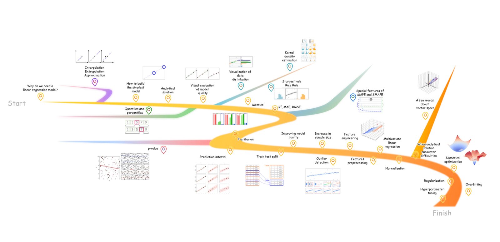
individuals! When you have ever wished to grasp how linear regression works or simply refresh the primary concepts with out leaping between a lot of totally different sources – this text is for you. It’s an additional lengthy learn that took me greater than a yr to write down. It’s constructed round 5 key concepts:

1. Visuals first. This can be a comic-style article: studying the textual content helps, however it’s not required. A fast run via the photographs and animations can nonetheless offer you a stable understanding of how issues work. There are 100+ visuals in complete;
2. Animations the place they could assist (33 complete). Laptop science is greatest understood in movement, so I take advantage of animations to clarify key concepts;
3. Newbie-friendly. I stored the fabric so simple as attainable, to make the article simple for learners to observe.
4. Reproducible. Most visuals had been generated in Python, and the code is open supply.
5. Give attention to observe. Every subsequent step solves an issue that exhibits up within the earlier step, so the entire article stays linked.

Another factor: the submit is simplified on function, so some wording and examples could also be a bit tough or not completely exact. Please don’t simply take my phrase for it – suppose critically and double-check my factors. For an important elements, I present hyperlinks to the supply code so you’ll be able to confirm every thing your self.

Desk of contents

Who’s this text for

Skip this paragraph, simply scroll via the article for 2 minutes and have a look at the visuals. You’ll instantly know if you wish to learn it correctly (the primary concepts are proven within the plots and animations). This submit is for learners and for anybody working with information – and in addition for skilled individuals who need a fast refresh.

What this submit covers

The article is structured in three acts:

• Linear regression: what it’s, why we use it, and how you can match a mannequin;
• The right way to consider the mannequin’s efficiency;
• The right way to enhance the mannequin when the outcomes usually are not ok.

At a excessive stage, this text covers:

1. data-driven modeling;
2. analytical resolution for linear regression, and why it isn’t all the time sensible;
3. methods to guage mannequin high quality, each visually and with metrics;
4. A number of linear regression, the place predictions are based mostly on many options;
5. the probabilistic aspect of linear regression, since predictions usually are not precise and you will need to quantify uncertainty;
6. methods to enhance mannequin high quality, from including complexity to simplifying the mannequin with regularization.

Extra particularly, it walks via:

1. the least squares technique for easy linear regression;
2. regression metrics reminiscent of R², RMSE, MAE, MAPE, SMAPE, together with the Pearson correlation coefficient and the coefficient of willpower, plus visible diagnostics like residual plots;
3. most chance and prediction intervals;
4. practice/take a look at splits, why they matter and how you can do them;
5. outlier dealing with strategies, together with RANSAC, Mahalanobis distance, Native Outlier Issue (LOF), and Cook dinner’s distance;
6. information preprocessing, together with normalization, standardization, and categorical encoding;
7. the linear algebra behind least squares, and the way it extends to multivariate regression;
8. numerical optimization strategies, together with gradient descent;
9. L1 and L2 regularization for linear fashions;
10. cross-validation and hyperparameter optimization.

Though this text focuses on linear regression, some elements – particularly the part on mannequin analysis, apply to different regression algorithms as effectively. The identical goes for the characteristic preprocessing chapters.

Since that is meant as an introductory, ML-related information to linear regression, I’ll largely keep away from vector notation (the place formulation use vectors as a substitute of scalars). In different phrases, you’ll hardly see vectors and matrices within the equations, besides in a couple of locations the place they’re actually vital. Take into account that many of the formulation proven right here do have a vector type, and trendy libraries implement the algorithms in precisely that manner. These implementations are environment friendly and dependable, so should you determine to code issues up, don’t reinvent the wheel – use well-tested libraries or instruments with UI when it is sensible.

All animations and pictures within the article are unique and created by the writer.

A short literary evaluate

This subject isn’t new, so there’s loads of materials on the market. Under is a brief record of direct predecessors, comparable in platform (largely In direction of Knowledge Science) and viewers, which means browser-first readers fairly than textbook readers. The record is ordered by rising subjective complexity:

• What’s Linear Regression? – A beginner-friendly overview of what linear regression is, what the road represents, how predictions are made, with easy visuals and code;
• A Sensible Information to Linear Regression – Represents linear mannequin becoming as machine studying pipeline: EDA, characteristic dealing with, mannequin becoming, and analysis on an actual Kaggle dataset;
• Mastering the Fundamentals: How Linear Regression Unlocks the Secrets and techniques of Advanced Fashions – Simple to observe information with step-by-step calculations memorable and good visuals;
• Predict Housing Value utilizing Linear Regression in Python – implementation-oriented article constructed across the Boston Housing dataset, with code examples for calculations from scratch; 
• A number of Linear Regression Evaluation – An article with extra mathematical element, targeted on multicollinearity;
• Mastering Linear Regression: The Definitive Information For Aspiring Knowledge Scientists – A protracted, multi function information, concept plus Python;
• Linear Regression In Depth (Half 1) and Linear Regression In Depth (Half 2)  – Deeper concept plus implementation articles that focuses on easy linear regression and units up the transition to a number of regression;

And naturally, don’t ignore the basic papers if you wish to learn extra about this subject. I’m not itemizing them as a separate bibliography on this part, however you’ll discover hyperlinks to them later within the textual content. Every reference seems proper after the fragment it pertains to, in sq. brackets, within the format: [Author(s). Title. Year. Link to the original source]

mannequin begins with information

Let’s assume we have now tabular information with two columns:

• Variety of rooms within the house;
• The worth of the house, $

By the point you construct a mannequin, there ought to already be information. Knowledge assortment and the preliminary preparation of the dataset are exterior the scope of this text, particularly because the course of can fluctuate lots relying on the area. The primary precept to bear in mind is “garbage in, garbage out,” which applies to supervised machine studying normally. mannequin begins with an excellent dataset.

Disclaimer relating to the dataset: The info used on this article is artificial and was generated by the writer. It’s distributed underneath the identical license because the supply code – BSD 3-Clause.

Why do we’d like a mannequin?

Because the British statistician George Field as soon as mentioned, “All models are wrong, but some are useful.” Fashions are helpful as a result of they assist us uncover patterns in information. As soon as these patterns are expressed as a mathematical relationship (a mannequin), we are able to use it, for instance, to generate predictions (Determine 2).

Modeling relationships in information just isn’t a trivial activity. It may be completed utilizing mathematical fashions of many alternative varieties – from easy ones to trendy multi-stage approaches reminiscent of neural networks. For now, the important thing level is {that a} “model” can imply any form of mapping from one set of knowledge (characteristic columns) to a goal column. I’ll use this definition all through the article.

In linear regression, we mannequin linear relationships between information variables. In pair (one-feature) regression – when there’s one characteristic and one dependent variable – the equation has the shape:

$y = b_0 + b_1 cdot x$, the place $x$ – characteristic, $y$ – goal variable [James, G., et al. Linear Regression. An Introduction to Statistical Learning, 2021. Free version https://www.statlearning.com/].

So the expression $y= 1 + 10cdot x$ is a linear regression mannequin. And $y = 15 − 21 cdot x$ is one as effectively – the one distinction is the coefficients. For the reason that coefficients are the important thing parameters of the equation, they’ve their very own names:

• b₀ – the intercept (additionally referred to as the bias time period)
• b₁ – the slope coefficient

So, once we construct a linear regression mannequin, we make the next assumption:

Assumption 1. The connection between the options (unbiased variables) and the response (dependent variable) is linear [Kim, Hae-Young. Statistical notes for clinical researchers: simple linear regression 1 – basic concepts, 2018.

An example of a linear model with the intercept and slope coefficients already fitted (we will discuss why they are called that a bit later) is shown in Figure 4.

For the dataset shown in Figure 1, estimating the apartment price in dollars means multiplying the number of rooms by 10 000. 

Important note: we are focusing on an approximation – so the model line does not have to pass through every data point, because real-world data almost never falls exactly on a single straight line. There is always some noise, and some factors the model does not see. It’s enough for the model line to stay as close to the observed data as possible. If you do not remember well the difference between approximation, interpolation and extrapolation, please check the image below. 

Side branch 1. Difference between approximation, interpolation and extrapolation

---

How to build a simple model

We need to choose the coefficients $b_0$ ​and $b_1$ ​in the equation below so that the straight line fits the empirical observations (the real data) as closely as possible: $y = b_0 + b_1 cdot x$, where $x$ – number of rooms, $y$ – apartment price, $.

Why this equation, and why two coefficients

Despite its apparent simplicity, the linear regression equation can represent many different linear relationships, as shown in Figure 5. For each dataset, a different line will be optimal.

Analytical solution

To find the optimal coefficient values, we will use an analytical solution: plug the empirical data from the previous section into a well-known formula derived long ago (by Carl Gauss and Adrien-Marie Legendre). The analytical solution can be written as four simple steps (Figure 6) [Hastie, T., et al. Linear Methods for Regression (Chapter 3 in The Elements of Statistical Learning: Data Mining, Inference, and Prediction). 2009. https://hastie.su.domains/ElemStatLearn].

Error can be a part of the mannequin

Earlier, I famous that linear regression is an approximation algorithm. This implies we don’t require the road to move precisely via the observations. In different phrases, even at this stage we enable the mannequin’s predictions to vary from the noticed house costs. And you will need to emphasize: this sort of mismatch is totally regular. In the true world, it is vitally exhausting to discover a course of that generates information mendacity completely on a straight line (Determine 7).

So, the mannequin wants yet another element to be life like: an error time period. With actual information, error evaluation is important – it helps spot issues and repair them early. Most significantly, it gives a approach to quantify how good the mannequin actually is.

The right way to measure mannequin high quality

Mannequin high quality may be assessed utilizing two essential approaches:

• Visible analysis
• Metric-based analysis

Earlier than we dive into every one, it’s a good second to outline what we imply by “quality” right here. On this article, we’ll contemplate a mannequin an excellent one when the error time period is as small as attainable.

Utilizing the unique dataset (see Determine 1), totally different coefficient values may be plugged into the linear regression equation. Predictions are then generated for the identified examples, and the distinction between predicted and precise values is in contrast (Desk 1). Amongst all combos of the intercept and slope, one pair yields the smallest error.

Variety of rooms	Mannequin (b0 + b1 x rooms quantity)	Prediction	Floor fact (commentary)	Error (commentary – predicted)
2	$0 + 10000 cdot 2$	20 000	20 000	0
2	$0 + 5000 cdot 2$	10 000	20 000	10 000
2	$500 + 1000 cdot 2$	2 500	20 000	17 500

The desk instance above is straightforward to observe as a result of it’s a small, toy setup. It solely exhibits how totally different fashions predict the worth of a two-room house, and within the unique dataset every “number of rooms” worth maps to a single worth. As soon as the dataset will get bigger, this sort of guide comparability turns into impractical. That’s why mannequin high quality is often assessed with analysis instruments (visuals, metrics and statistical exams) fairly than hand-made tables.

To make issues a bit extra life like, the dataset can be expanded in three variations: one simple case and two which can be tougher to suit. The identical analysis will then be utilized to those datasets.

Determine 8 is nearer to actual life: flats fluctuate, and even when the variety of rooms are the identical, the worth throughout totally different properties doesn’t must be similar.

Visible analysis

Utilizing the components from the Analytic Resolution part (Determine 6), the info may be plugged in to acquire the next fashions for every dataset:

1. A: $0 + 10000 cdot x$, the place x is rooms quantity
2. B: $0 + 10000 cdot x$, the place x is rooms quantity
3. C: $6800 + 6600 cdot x$, the place x is rooms quantity

A helpful first plot to indicate right here is the scatter plot: the characteristic values are positioned on the x-axis, whereas the y-axis exhibits each the anticipated values and the precise observations, in several colours. This type of determine is simple to interpret – the nearer the mannequin line is to the true information, the higher the mannequin. It additionally makes the connection between the variables simpler to see, because the characteristic itself is proven on the plot [Piñeiro, G., et al. How to evaluate models: Observed vs. predicted or predicted vs. observed? 2008. https://doi.org/10.1016/j.ecolmodel.2008.05.006].

One draw back of this plot is that it turns into exhausting to introduce further options after you have a couple of or two – for instance, when worth relies upon not solely on the variety of rooms, but additionally on the gap to the closest metro station, the ground stage, and so forth. One other situation is scale: the goal vary can strongly form the visible impression. Tiny variations on the chart, barely seen to the attention, should correspond to errors of a number of thousand {dollars}. Value prediction is a superb instance right here, as a result of a deceptive visible impression of mannequin errors can translate immediately into cash.

When the variety of options grows, visualizing the mannequin immediately (characteristic vs. goal with a fitted line) rapidly turns into messy. A cleaner various is an noticed vs. predicted scatter plot. It’s constructed like this: the x-axis exhibits the precise values, and the y-axis exhibits the anticipated values (Determine 10) [Moriasi, D. N., et al. Hydrologic and Water Quality Models: Performance Measures and Evaluation Criteria. 2015. pdf link]. I’ve additionally seen the axes swapped, with predicted values on the x-axis as a substitute. Both manner, the plot serves the identical function – so be happy to decide on whichever conference you like.

This plot is learn as follows: the nearer the factors are to the diagonal line coming from the bottom-left nook, the higher. If the mannequin reproduced the observations completely, each level would sit precisely on that line with none deviation (dataset A appears to be like fairly near this superb case).

When datasets are giant, or the construction is uneven (for instance, when there are outliers), Q-Q plots may be useful. They present the identical predicted and noticed values on the identical axes, however after a particular transformation.

Q-Q plot Possibility 1, – order statistics. Predicted values are sorted in ascending order, and the identical is completed for the noticed values. The 2 sorted arrays are then plotted towards one another, similar to in Determine 10.

Q-Q plot Possibility 2, – two-sample Q-Q plot. Right here the plot makes use of quantiles fairly than uncooked sorted values. The info are grouped right into a finite variety of ranges (I often use round 100). This plot is helpful when the purpose is to check the general sample, not particular person “prediction vs. observation” pairs. It helps to see the form of the distributions, the place the median sits, and the way frequent very giant or very small values are.

Facet department 2. Reminder about quantiles

In line with Wikipedia, a quantile is a worth {that a} given random variable doesn’t exceed with a set likelihood.

Setting the likelihood wording apart for a second, a quantile may be regarded as a worth that splits a dataset into elements. For instance, the 0.25 quantile is the quantity under which 25% of the pattern lies. And the 0.9 quantile is the worth under which 90% of the info lies.

For the pattern [ 1 , 3 , 5 , 7 , 9 ] the 0.5 quantile (the median) is 5. There are solely two values above 5 (7 and 9), and solely two under it (1 and three). 

The 0.25 quantile is roughly 3, and the 0.75 quantile is roughly 7. See the reason within the determine under.

The 25^th percentile can be referred to as the primary quartile, the 50^th percentile is the median or second quartile, and the 75^th percentile is the third quartile.

---

Within the second variant, irrespective of how giant the dataset is, this plot all the time exhibits 99 factors, so it scales effectively to giant samples. In Determine 11, the true and predicted quantiles for dataset A lie near the diagonal line which signifies an excellent mannequin. For dataset B, the fitting tail of the distributions (upper-right nook) begins to diverge, which means the mannequin performs worse on high-priced flats.

For dataset C: 

• Under the 25^th percentile, the anticipated quantiles lie above the noticed ones;
• Inside the interquartile vary (from the 25^th to the 75^th percentile), the anticipated quantiles lie under the noticed ones;
• Above the 75^th percentile, the anticipated tail once more lies above the noticed one.

One other broadly used diagnostic is the residual plot. The x-axis exhibits the anticipated values, and the y-axis exhibits the residuals. Residuals are the distinction between the noticed and predicted values. If you happen to choose, you’ll be able to outline the error with the alternative signal (predicted minus noticed) and plot that as a substitute. It doesn’t change the concept – solely the path of the values on the y-axis.

A residual plot is likely one of the most handy instruments for checking the important thing assumptions behind linear regression (Assumption 1 (linearity) was launched earlier):

• Assumption 2. Normality of residuals. The residuals (noticed minus predicted) needs to be roughly usually distributed. Intuitively, most residuals needs to be small and near zero, whereas giant residuals are uncommon. Residuals happen roughly equally typically within the optimistic and unfavorable path.
• Assumption 3. Homoscedasticity (fixed variance). The mannequin ought to have errors of roughly the identical magnitude throughout the complete vary: low cost flats, mid-range ones, and costly ones.
• Assumption 4. Independence. Observations (and their residuals) needs to be unbiased of one another – i.e., there needs to be no autocorrelation.

Determine 12 exhibits that dataset B violates Assumption 3: because the variety of rooms will increase, the errors get bigger – the residuals fan out from left to proper, indicating rising variance. In different phrases, the error just isn’t fixed and will depend on the characteristic worth. This often means the mannequin is lacking some underlying sample, which makes its predictions much less dependable in that area.

For dataset C, the residuals don’t look regular: the mannequin typically systematically overestimates and typically systematically underestimates, so the residuals drift above and under zero in a structured manner fairly than hovering round it randomly. On high of that, the residual plot exhibits seen patterns, which could be a signal that the errors usually are not unbiased (to be truthful, not all the time XD however both manner it’s a sign that one thing is off with the mannequin).

A pleasant companion to Determine 12 is a set of residual distribution plots (Determine 13). These make the form of the residuals instantly seen: even with out formal statistical exams, you’ll be able to eyeball how symmetric the distribution is (an excellent signal is symmetry round zero) and the way heavy its tails are. Ideally, the distribution ought to look bell-shaped, most residuals needs to be small, whereas giant errors needs to be uncommon.

Facet department 3. A fast reminder about frequency distributions

In case your stats course has pale from reminiscence otherwise you by no means took one this half is price a more in-depth look. This part introduces the most typical methods to visualise samples in mathematical statistics. After it, deciphering the plots used later within the article needs to be simple.

Frequency distribution is an ordered illustration displaying what number of occasions the values of a random variable fall inside sure intervals.

To construct one:

1. Cut up the complete vary of values into okay bins (class intervals)
2. Depend what number of observations fall into every bin – this is absolutely the frequency
3. Divide absolutely the frequency by the pattern measurement n to get the relative frequency

Within the determine under, the identical steps are proven for the variable V:

The identical form of visualization may be constructed for variable U as effectively, however on this part the main target stays on V for simplicity. Afterward, the histogram can be rotated sideways to make it simpler to check the uncooked information with the vertical format generally used for distribution plots.

From the algorithm description and from the determine above, one vital disadvantage turns into clear: the variety of bins okay (and subsequently the bin width) has a serious affect on how the distribution appears to be like.

There are empirical formulation that assist select an inexpensive variety of bins based mostly on the pattern measurement. Two frequent examples are Sturges’ rule and the Rice rule (see Additional Determine 5 under) [Sturges. The Choice of a Class Interval. 1926. DOI: 10.1080/01621459.1926.10502161], [Lane, David M., et. al. Histograms. https://onlinestatbook.com/2/graphing_distributions/histograms.html].

Another is to visualise the distribution utilizing kernel density estimation (KDE). KDE is a smoothed model of a histogram: as a substitute of rectangular bars, it makes use of a steady curve constructed by summing many {smooth} “kernel” features, often, regular distributions (Additional Determine 6).

I perceive that describing KDE as a sum of “tiny normal distributions” isn’t very intuitive. Right here’s a greater psychological image. Think about that every information level is crammed with numerous tiny grains of sand. If you happen to let the sand fall underneath gravity, it types somewhat pile immediately beneath that time. When a number of factors are shut to one another, their sand piles overlap and construct a bigger mound. Watch the animation under to see the way it works:

In a KDE plot, these “sand piles” are sometimes modeled as small regular (Gaussian) distributions positioned round every information level.

One other broadly used approach to summarize a distribution is a field plot. A field plot describes the distribution by way of quartiles. It exhibits:

• The median (second quartile, Q2);
• The primary (Q1) and third (Q3) quartiles (the twenty fifth and seventy fifth percentiles), which type the perimeters of the “box”;
• The whiskers, which mark the vary of the info excluding outliers;
• Particular person factors, which characterize outliers.

To sum up, the subsequent step is to visualise samples of various styles and sizes utilizing all of the strategies mentioned above. This can be completed by drawing samples from totally different theoretical distributions: two pattern sizes for every, 30 and 500 observations.

A frequency distribution is a key instrument for describing and understanding the habits of a random variable based mostly on a pattern. Visible strategies like histograms, kernel density curves, and field plots complement one another and assist construct a transparent image of the distribution: its symmetry, the place the mass is concentrated, how unfold out it’s, and whether or not it comprises outliers.

Such viewpoint on the info can be helpful as a result of it has a pure probabilistic interpretation: the more than likely values fall within the area the place the likelihood density is highest, i.e., the place the KDE curve reaches its peak.

---

As famous above, the residual distribution ought to look roughly regular. That’s why it is sensible to check two distributions: theoretical regular vs. the residuals we truly observe. Two handy instruments for this are density plots and Q-Q plots with residual quantiles vs. regular quantiles. The parameters of the conventional distribution are estimated from the residual pattern. Since these plots work greatest with bigger samples, for illustration I’ll artificially improve every residual set to 500 values whereas preserving the important thing habits of the residuals for every dataset (Determine 14).

As Determine 14 exhibits, the residual distributions for datasets A* and B* are moderately effectively approximated by a standard distribution. For B*, the tails drift a bit: giant errors happen barely extra typically than we wish. The bimodal case C* is rather more hanging: its residual distribution appears to be like nothing like regular.

Heteroscedasticity in B* gained’t present up in these plots, as a result of they have a look at residuals on their very own (one dimension) and ignore how the error adjustments throughout the vary of predictions.

To sum up, a mannequin is never excellent, it has errors. Error evaluation with plots is a handy approach to diagnose the mannequin:

• For pair regression, it’s helpful to plot predicted and noticed values on the y-axis towards the characteristic on the x-axis. This makes the connection between the characteristic and the response simple to see;
• As an addition, plot noticed values (x-axis) vs. predicted values (y-axis). The nearer the factors are to the diagonal line coming from the bottom-left nook, the higher. This plot can be useful as a result of it doesn’t depend upon what number of options the mannequin has;
• If the purpose is to check the complete distributions of predictions and observations, fairly than particular person pairs, a Q-Q plot is an efficient alternative;
• For very giant samples, cognitive load may be decreased by grouping values into quantiles on the Q-Q plot, so the plot can have, for instance, solely 100 scatter factors;
• A residual plot helps examine whether or not the important thing linear regression assumptions maintain for the present mannequin (independence, normality of residuals, and homoscedasticity);
• For a better comparability between the residual distribution and a theoretical regular distribution, use a Q-Q plot.

Metrics

Disclaimer relating to the designations X and Y

Within the visualizations on this part, some notation could look a bit uncommon in comparison with associated literature. For instance, predicted values are labeled $X$, whereas the noticed response is labeled $Y$. That is intentional: despite the fact that the dialogue is tied to mannequin analysis, I don’t need it to really feel like the identical concepts solely apply to the “prediction vs. observation” pair. In observe, $X$ and $Y$ may be any two arrays – the fitting alternative will depend on the duty.

There’s additionally a sensible cause for selecting this pair: $X$ and $Y$ are visually distinct. In plots and animations, they’re simpler to inform aside than pairs like $U$ and $V$, or the extra acquainted $y$ and $hat{y}$.

---

As compelling as visible diagnostics may be, mannequin high quality is greatest assessed along with metrics (numerical measures of efficiency). metric is interesting as a result of it reduces cognitive load: as a substitute of inspecting yet one more set of plots, the analysis collapses to a single quantity (Determine 15).

In contrast to a residual plot, a metric can be a really handy format for automated evaluation, not simply simple to interpret, however simple to plug into code. That makes metrics helpful for numerical optimization, which we’ll get to a bit later.

This “Metrics” part additionally contains statistical exams: they assist assess the importance of particular person coefficients and of the mannequin as an entire (we’ll cowl that later as effectively).

Here’s a non-exhaustive record:

• Coefficient of willpower R² – [Kvalseth, Tarald O. Cautionary Note about R². 1985. https://www.tandfonline.com/doi/abs/10.1080/00031305.1985.10479448];
• Bias;
• Imply absolute error – MAE;
• Root imply sq. error – RMSE;
• Imply absolute share error – MAPE;
• Symmetric imply absolute share error – SMAPE;
• The F-test for checking whether or not the mannequin is critical as an entire;
• The t-test for checking the importance of the options and the goal;
• Durbin-Watson take a look at for analyzing residuals.

Determine 16 exhibits metrics computed by evaluating the noticed house costs with the anticipated ones.

The metrics are grouped for readability. The primary group, proven in crimson, contains the correlation coefficient (between predicted and noticed values) and the coefficient of willpower, R². Each are dimensionless, and values nearer to 1 are higher. Notice that correlation just isn’t restricted to predictions versus the goal. It can be computed between a characteristic and the goal, or pairwise between options when there are numerous of them.

The second group, proven in inexperienced, contains metrics that measure error in the identical items because the response, which right here means $. For all three metrics, the interpretation is identical: the nearer the worth is to zero, the higher (Animation 2).

One fascinating element: in Determine 16 the bias is zero in all instances. Actually, this implies the mannequin errors usually are not shifted in both path on common. A query for you: why is that this usually true for a linear regression mannequin fitted to any dataset (attempt altering the enter values and enjoying with totally different datasets)?

Animation 2 and Determine 16 additionally present that because the hole between $X$ and $Y$ grows, RMSE reacts extra strongly to giant errors than MAE. That occurs as a result of RMSE squares the errors.

The third group, proven in blue, contains error metrics measured in percentages. Decrease values are higher. MAPE is delicate to errors when the true values are small, as a result of the components divides the prediction error by the noticed worth itself. When the precise worth is small, even a modest absolute error turns into a big share and might strongly have an effect on the ultimate rating (Determine 17).

Determine 17 exhibits that the distinction measured within the unique items, absolutely the deviation between noticed and predicted values, stays the identical in each instances: it’s 0 for the primary pair, 8 for the second, and 47 for the third. For percentage-based metrics, the errors shrink for an apparent cause: the noticed values grow to be bigger.

The change is bigger for MAPE, as a result of it normalizes every error by the noticed worth itself. sMAPE, in distinction, normalizes by the typical magnitude of the noticed and predicted values. This distinction issues most when the observations are near zero, and it fades as values transfer away from zero, which is strictly what the determine exhibits.

Facet department 4. Options of MAPE and SMAPE calculations

The small print of metric calculations are vital to debate. Utilizing MAPE and SMAPE (and briefly MAE) as examples, this part exhibits how otherwise metrics can behave throughout datasets. The primary takeaway is straightforward: earlier than beginning any machine studying challenge, think twice about which metric, or metrics, it is best to use to measure high quality. Not each metric is an efficient match in your particular activity or information.

Here’s a small experiment. Utilizing the info from Determine 17, take the unique arrays, observations [1,2,3] and predictions [1,10,50]. Shift each arrays away from zero by including 10 to each worth, repeated for 10 iterations. At every step, compute three metrics: MAPE, SMAPE, and MAE. The outcomes are proven within the plot under:

As may be seen from the determine above, the bigger the values included within the dataset, the smaller the distinction between MAPE and SMAPE, and the smaller the errors measured in share phrases. The alignment of MAPE and SMAPE is defined by the calculation options that enable eliminating the impact of MAPE asymmetry, which is especially noticeable at small commentary values. MAE stays unchanged, as anticipated.

Now the explanation for the phrase “asymmetry” turns into clear. The best approach to present it’s with an instance. Suppose the mannequin predicts 110 when the true worth is 100. In that case, MAPE is 10%. Now swap them: the true worth is 110, however the prediction is 100. Absolutely the error remains to be 10, but MAPE turns into 9.1%. MAPE is uneven as a result of the identical absolute deviation is handled otherwise relying on whether or not the prediction is above the true worth or under it.

One other disadvantage of MAPE is that it can’t be computed when some goal values are zero. A standard workaround is to switch zeros with a really small quantity throughout analysis, for instance 0.000001. Nonetheless, it’s clear that this could inflate MAPE.

Different metrics have their very own quirks as effectively. For instance, RMSE is extra delicate to giant errors than MAE. This part just isn’t meant to cowl each such element. The primary level is straightforward: select metrics thoughtfully. Use metrics really useful in your area, and if there are not any clear requirements, begin with the most typical ones and experiment.

---

To summarize, the items of measurement for metrics and the ranges of attainable values are compiled in Desk 2.

Metric	Items	Vary	Which means
Pearson correlation coefficient (predictions vs goal)	Dimensionless	from -1 to 1	The nearer to 1, the higher the mannequin
Coefficient of willpower R2	Dimensionless	from −∞ to 1	The nearer to 1, the higher the mannequin
Bias	The identical unit because the goal variable	from −∞ to ∞	The nearer to 1, the higher the mannequin
Imply absolute error (MAE)	The identical unit because the goal variable	from 0 to ∞	The nearer to zero, the higher the mannequin
Root imply sq. error (RMSE)	The identical unit because the goal variable	from 0 to ∞	The nearer to zero, the higher the mannequin
Imply absolute share error (MAPE)	Share (%)	from 0 to ∞	The nearer to zero, the higher the mannequin
Symmetric imply absolute share error (SMAPE)	Share (%)	from 0 to 200	The nearer to zero, the higher the mannequin

As talked about earlier, this isn’t a whole record of metrics. Some duties could require extra specialised ones. If wanted, fast reference information is all the time simple to get out of your favourite LLM.

Here’s a fast checkpoint. Mannequin analysis began with a desk of predicted and noticed values (Desk 1). Giant tables are exhausting to examine, so the identical data was made simpler to digest with plots, shifting to visible analysis (Figures 9-14). The duty was then simplified additional: as a substitute of counting on professional judgment from plots, metrics had been computed (Figures 15-17 and Animations 1-3). There’s nonetheless a catch. Even after getting one or a number of numbers, it’s nonetheless as much as us to determine whether or not the metric worth is “good” or not. In Determine 15, a 5% threshold was used for MAPE. That heuristic can’t be utilized to each linear regression activity. Knowledge varies, enterprise objectives are totally different, and so on. For one dataset, an excellent mannequin would possibly imply an error under 7.5%. For one more, the suitable threshold is likely to be 11.2%.

F take a look at

That’s the reason we now flip to statistics and formal speculation testing. A statistical take a look at can, in precept, save us from having to determine the place precisely to put the metric threshold, with one vital caveat, and provides us a binary reply: sure or no.

When you have by no means come throughout statistical exams earlier than, it is sensible to begin with a simplified definition. A statistical take a look at is a approach to examine whether or not what we observe is simply random variation or an actual sample. You may consider it as a black field that takes in information and, utilizing a set of formulation, produces a solution: a couple of intermediate values, reminiscent of a take a look at statistic and a p-value, and a ultimate verdict (Determine 18) [Sureiman, Onchiri, et al. F-test of overall significance in regression analysis simplified. 2020. https://www.tandfonline.com/doi/full/10.1080/00031305.2016.1154108].

As Determine 18 exhibits, earlier than working a take a look at, we have to select a threshold worth. Sure, that is the fitting second to come back again to that caveat: right here too, we have now to cope with a threshold. However on this case it’s a lot simpler, as a result of there are broadly accepted commonplace values to select from. This threshold is named the importance stage. A worth of 0.05 signifies that we settle for a 5% likelihood of incorrectly rejecting the null speculation. On this case, the null speculation might be one thing like: the mannequin isn’t any higher than a naive prediction based mostly on the imply. We are able to fluctuate this threshold. For instance, some scientific fields use 0.01 and even 0.001, which is extra strict, whereas others use 0.10, which is much less strict.

If the sensible which means of the importance stage just isn’t absolutely clear at this level, that’s utterly tremendous. There’s a extra detailed rationalization on the finish of this part. For now, it is sufficient to repair one key level: the statistical exams mentioned under have a parameter, $alpha$, which we as researchers or engineers select based mostly on the duty. In our case, it’s set to 0.05.

So, a statistical take a look at lets us take the info and some chosen parameters, then compute take a look at portions which can be used for comparability, for instance, whether or not the take a look at statistic is above or under a threshold. Primarily based on that comparability, we determine whether or not the mannequin is statistically vital. I might not advocate reinventing the wheel right here. It’s higher to make use of statistical packages (it’s dependable) to compute these exams, which is one cause why I’m not giving the formulation on this part. As for what precisely to check, the 2 frequent choices are the F statistic towards the important F worth, or the p-value towards the importance stage. Personally, largely out of behavior, I lean towards the second possibility.

We are able to use the F take a look at to reply the query, “Is the model significant?” Since statistics is a mathematical self-discipline, allow us to first describe the 2 attainable interpretations of the fitted mannequin in a proper manner. The statistical take a look at will assist us determine which of those hypotheses is extra believable.

We are able to formulate the null speculation (H₀) as follows: all coefficients for the unbiased variables, that’s, the options, are equal to zero. The mannequin doesn’t clarify the connection between the options and the goal variable any higher than merely utilizing the (goal) imply worth.

The choice speculation (H₁) is then: not less than one coefficient just isn’t equal to zero. In that case, the mannequin is critical as a result of it explains some a part of the variation within the goal variable.

Now allow us to run the exams on our three datasets, A, B, and C (Determine 19).

As we are able to see from Determine 19, in all three instances the p-value is under 0.05, which is our chosen significance stage. We use 0.05 as a result of it’s the usual default threshold, and within the case of house worth prediction, selecting the incorrect speculation just isn’t as important as it could be, for instance, in a medical setting. So there isn’t a robust cause to make the brink extra strict right here. p-value is under 0.05 means we reject the null speculation, H₀, for fashions A, B, and C. After this examine, we are able to say that each one three fashions are statistically vital total: not less than one characteristic contributes to explaining variation within the goal.

Nevertheless, the instance of dataset C exhibits that affirmation that the mannequin is considerably higher than the typical worth doesn’t essentially imply that the mannequin is definitely good. The F-statistic checks for minimal adequacy.

One limitation of this method to mannequin analysis is that it’s fairly slender in scope. The F take a look at is a parametric take a look at designed particularly for linear fashions, so not like metrics reminiscent of MAPE or MAE, it can’t be utilized to one thing like a random forest (one other machine studying algorithm). Even for linear fashions, this statistical take a look at additionally requires commonplace assumptions to be met (see Assumptions 2-4 above: independence of observations, normality of residuals, and homoscedasticity).

Nonetheless, if this subject pursuits you, there’s loads extra to discover by yourself. For instance, you would look into the t take a look at for particular person options, the place the speculation is examined individually for every mannequin coefficient, or the Durbin-Watson take a look at. Or you’ll be able to select another statistical take a look at to check additional. Right here we solely coated the fundamental concept. P.S. It’s particularly price taking note of how the take a look at statistics are calculated and to the mathematical instinct behind them.

Facet department 5. If you’re not solely clear in regards to the significance stage $alpha$, please learn this part

Each time I attempted to grasp what significance stage meant, I ran right into a brick wall. Extra complicated examples concerned calculations that I didn’t perceive. Easier sources conveyed the idea extra clearly – “here’s an example where everything is intuitively understandable”:

• H₀ (null speculation): The affected person doesn’t have most cancers;
• Sort I error: The take a look at says “cancer is present” when it isn’t truly;
• If the importance stage $alpha$ is ready at 0.05, in 5% of instances the take a look at could mistakenly alarm a wholesome individual by informing them that they’ve most cancers;
• Due to this fact, in drugs, a low $alpha$ (e.g., 0.01) is commonly chosen to reduce false alarms.

However right here we have now information and mannequin coefficients – every thing is fastened. We apply the F-test and get a p-value < 0.05. We are able to run this take a look at 100 occasions, and the end result would be the identical, as a result of the mannequin is identical and the coefficients are the identical. There we go – 100 occasions we get affirmation that the mannequin is critical. And what’s the 5 p.c threshold right here? The place does this “probability” come from?

Allow us to break this down collectively. Begin with the phrase, “The model is significant at the 0.05 level”. Regardless of the way it sounds, this phrase just isn’t actually in regards to the mannequin itself. It’s actually a press release about how convincing the noticed relationship is within the information we used. In different phrases, think about that we repeatedly gather information from the true world, match a mannequin, then gather a brand new pattern and match one other one, and preserve doing this many occasions. In a few of these instances, we’ll nonetheless discover a statistically vital relationship even when, in actuality, no actual relationship exists between the variables. The importance stage helps us account for that.

To sum up, with a p-value threshold of 0.05, even when no actual relationship exists, the take a look at will nonetheless say “there is a relationship” in about 5 out of 100 instances, merely due to random variation within the information.

To make the textual content a bit much less dense, let me illustrate this with an animation. We’ll generate 100 random factors, then repeatedly draw datasets of 30 observations from that pool and match a linear regression mannequin to every one. We’ll repeat this sampling course of 20 occasions. With a significance stage of 5%, this implies we enable for about 1 case out of 20 during which the F take a look at says the mannequin is critical despite the fact that, in actuality, there isn’t a relationship between the variables.

Certainly, in 1 out of 20 instances the place there was truly no relationship between x and y, the take a look at nonetheless produced a p-value under 0.05. If we had chosen a stricter significance stage, for instance 0.01, we’d have prevented a Sort I error, that’s, a case the place we reject H₀ (there isn’t a relationship between x and y) and settle for the choice speculation despite the fact that H₀ is in reality true.

For comparability, we’ll now generate a inhabitants the place a transparent linear relationship is current and repeat the identical experiment: 20 samples and the identical 20 makes an attempt to suit a linear regression mannequin.

---

To wrap up this overview chapter on regression metrics and the F take a look at, listed below are the primary takeaways:

• Visible strategies usually are not the one approach to assess prediction error. We are able to additionally use metrics. Their essential benefit is that they summarize mannequin high quality in a single quantity, which makes it simpler to guage whether or not the mannequin is sweet sufficient or not.
• Metrics are additionally used throughout mannequin optimization, so you will need to perceive their properties. For instance:
  • The metrics from the “green group” (RMSE, MAE, and bias) are handy as a result of they’re expressed within the unique items of the goal.
  • The foundation imply squared error (RMSE) reacts extra strongly to giant errors and outliers than the imply absolute error (MAE).
  • The “blue group” (MAPE and SMAPE) is expressed in p.c, which frequently makes these metrics handy to debate in a enterprise context. On the identical time, when the goal values are near zero, these metrics can grow to be unstable and produce deceptive estimates.
• Statistical exams present an much more compact evaluation of mannequin high quality, giving a solution within the type of “yes or no”. Nevertheless, as we noticed above, such a take a look at solely checks fundamental adequacy, the place the primary various to the fitted regression mannequin is just predicting the imply. It doesn’t assist in extra complicated instances, reminiscent of dataset C, the place the connection between the characteristic and the goal is captured by the mannequin effectively sufficient to rise above statistical noise, however not absolutely.

Later within the article, we’ll use totally different metrics all through the visualizations, so that you simply get used to wanting past only one favourite from the record 🙂

Forecast uncertainty. Prediction interval

An fascinating mixture of visible evaluation and formal metrics is the prediction interval. A prediction interval is a spread of values inside which a brand new commentary is predicted to fall with a given likelihood. It helps present the uncertainty of the prediction by combining statistical measures with the readability of a visible illustration (Determine 20).

The primary query right here is how to decide on these threshold values, $Delta$. Essentially the most pure method, and the one that’s truly utilized in observe, is to extract details about uncertainty from the instances the place the mannequin already made errors throughout coaching, particularly from the residuals. However to show a uncooked set of variations into precise threshold values, we have to go one stage deeper and have a look at linear regression as a probabilistic mannequin.

Recall how level prediction works. We plug the characteristic values into the mannequin, within the case of straightforward linear regression, only one characteristic, and compute the prediction. However a prediction is never precise. Most often, there’s a random error.

After we arrange a linear regression mannequin, we assume that small errors are extra seemingly than giant ones, and that errors in both path are equally seemingly. These two assumptions result in the probabilistic view of linear regression, the place the mannequin coefficients and the error distribution are handled as two elements of the identical complete (Determine 21) [Fisher, R. A. On the Mathematical Foundations of Theoretical Statistics. 1922. https://doi.org/10.1098/rsta.1922.0009].

As Determine 21 exhibits, the variability of the mannequin errors may be estimated by calculating the usual deviation of the errors, denoted by $sigma$. We may additionally speak in regards to the error variance right here, since it’s one other appropriate measure of variability. The usual deviation $sigma$ is just the sq. root of the variance. The bigger the usual deviation, the better the uncertainty of the prediction (see Part 2 in Determine 21).

This leads us to the subsequent step within the logic: the extra broadly the errors are unfold, the much less sure the mannequin is, and the broader the prediction interval turns into. General, the width of the prediction interval will depend on three essential elements:

• Noise within the information: the extra noise there’s, the better the uncertainty;
• Pattern measurement: the extra information the mannequin has seen throughout coaching, the extra reliably its coefficients are estimated, and the narrower the interval turns into;
• Distance from the middle of the info: the farther the brand new characteristic worth is from the imply, the upper the uncertainty.

In simplified type, the process for constructing a prediction interval appears to be like like this:

1. We match the mannequin (utilizing the components from the earlier part, Determine 6)
2. We compute the error element, that’s, the residuals
3. From the residuals, we estimate the everyday measurement of the error
4. Acquire the purpose prediction
5. Subsequent, we scale s utilizing a number of adjustment elements: how a lot coaching information the mannequin was fitted on, how far the characteristic worth is from the middle of the info, and the chosen confidence stage. The boldness stage controls how seemingly the interval is to comprise the worth of curiosity. We select it based mostly on the duty, in a lot the identical manner we earlier selected the importance stage for statistical testing (frequent by default – 0.95).

As a easy instance, we’ll generate a dataset of 30 observations with a “perfect” linear relationship between the characteristic and the goal, match a mannequin, and compute the prediction interval. Then we’ll 1) add noise to the info, 2) improve the pattern measurement, and three) increase the arrogance stage from 90% to 95 and 99%, the place the prediction interval reaches its most width (see Animation 4).

And contemplate individually what the prediction interval appears to be like like for datasets A, B, and C (Determine 22).

Determine 22 clearly exhibits that despite the fact that fashions A and B have the identical coefficients, their prediction intervals differ in width, with the interval for dataset B being a lot wider. In absolute phrases, the widest prediction interval, as anticipated, is produced by the mannequin fitted to dataset C.

Practice take a look at break up and metrics  

The entire high quality assessments mentioned to this point targeted on how the mannequin behaves on the identical observations it was skilled on. In observe, nonetheless, we wish to know whether or not the mannequin may also carry out effectively on new information it has not seen earlier than.

That’s the reason, in machine studying, it is not uncommon greatest observe to separate the unique dataset into elements. The mannequin is fitted on one half, the coaching set, and its means to generalize is evaluated on the opposite half, the take a look at pattern (Determine 23).

If we mix these mannequin diagnostic strategies into one giant visualization, that is what we get:

Determine 24 exhibits that the metric values are worse on the take a look at information, which is strictly what we’d count on, because the mannequin coefficients had been optimized on the coaching set. A couple of extra observations stand out:

• First, the bias metric has lastly grow to be informative: on the take a look at information it’s now not zero, because it was on the coaching information, and now shifts in each instructions, upward for datasets A and B, and downward for dataset C.
• Second, dataset complexity clearly issues right here. Dataset A is the simplest case for a linear mannequin, dataset B is tougher, and dataset C is probably the most troublesome. As we transfer from coaching to check information, the adjustments within the metrics grow to be extra noticeable. The residuals additionally grow to be extra unfold out within the plots.

On this part, you will need to level out that the best way we break up the info into coaching and take a look at units can have an effect on what our mannequin appears to be like like (Animation 5).

The selection of splitting technique will depend on the duty and on the character of the info. In some instances, the subsets shouldn’t be fashioned at random. Listed below are a couple of conditions the place that is sensible:

• Geographic or spatial dependence. When the info have a spatial element, for instance temperature measurements, air air pollution ranges, or crop yields from totally different fields, close by observations are sometimes strongly correlated. In such instances, it is sensible to construct the take a look at set from geographically separated areas so as to keep away from overestimating mannequin efficiency.
• State of affairs-based testing. In some enterprise issues, you will need to consider upfront how the mannequin will behave in sure important or uncommon conditions, for instance at excessive or excessive characteristic values. Such instances may be deliberately included within the take a look at set, even when they’re absent or underrepresented within the coaching pattern.

Think about that there are solely 45 flats on the planet…

To make the remainder of the dialogue simpler to observe, allow us to introduce one vital simplification for this text. Think about that our hypothetical world, the one during which we construct these fashions, could be very small and comprises solely 45 flats. In that case, all our earlier makes an attempt to suit fashions on datasets A, B, and C had been actually simply particular person steps towards recovering that unique relationship from all of the obtainable information.

From this viewpoint, A, B, and C usually are not actually separate datasets, despite the fact that we are able to think about them as information collected in three totally different cities, A, B, and C. As an alternative, they’re elements of a bigger inhabitants, D. Allow us to assume that we are able to mix these samples and work with them as a single complete (Determine 25).

It is very important take into account that every thing we do, splitting the info into coaching and take a look at units, preprocessing the info, calculating metrics, working statistical exams, and every thing else, serves one purpose: to ensure the ultimate mannequin describes the complete inhabitants effectively. The purpose of statistics, and that is true for supervised machine studying as effectively, is to draw conclusions about the entire inhabitants utilizing solely a pattern.

In different phrases, if we someway constructed a mannequin that predicted the costs of those 45 flats completely, we’d have a instrument that all the time provides the proper reply, as a result of on this hypothetical world there are not any different information on which the mannequin may fail. Once more, every thing right here will depend on that “if.” Now let me return us to actuality and attempt to describe all the info with a single linear regression mannequin (Determine 26).

In the true world, gathering information on each house is bodily inconceivable, as a result of it could take an excessive amount of time, cash, and energy, so we all the time work with solely a subset. The identical applies right here: we collected samples and tried to estimate the connection between the variables in a manner that will convey us as shut as attainable to the connection in inhabitants, total dataset D.

One crucial notice: Later within the article, we’ll often benefit from the foundations of our simplified world and peek at how the fitted mannequin behaves on the complete inhabitants. It will assist us perceive whether or not our modifications had been profitable, when the error metric goes down, or not, when the error metric goes up. On the identical time, please take into account that this isn’t one thing we are able to do in the true world. In observe, it’s inconceivable to guage a mannequin on each single object!

Enhancing mannequin high quality

Within the earlier part, earlier than we mixed our information into one full inhabitants, we measured the mannequin’s prediction error and located the outcomes unsatisfying. In different phrases, we wish to enhance the mannequin. Broadly talking, there are 3 ways to do this: change the info, change the mannequin, or change each. Extra particularly, the choices are:

• Increasing the pattern: rising the variety of observations within the dataset
• Decreasing the pattern: eradicating outliers and different undesirable rows from the info desk
• Making the mannequin extra complicated: including new options, both immediately noticed or newly engineered
• Making the mannequin easier: lowering the variety of options (typically this additionally improves the metrics)
• Tuning the mannequin: trying to find the most effective hyperparameters, which means parameters that aren’t discovered throughout coaching

We’ll undergo these approaches one after the other, beginning with pattern growth. For example the concept, we’ll run an experiment.

Increasing the pattern

Take into account that the values from the complete inhabitants usually are not immediately obtainable to us, and we are able to solely entry them in elements. On this experiment, we’ll randomly draw samples of 10 and 20 flats. For every pattern measurement, we’ll repeat the experiment 30 occasions. The metrics can be measured on 1) the coaching set, 2) the take a look at set, and three) the inhabitants, that’s, all 45 observations. This could assist us see whether or not bigger samples result in a extra dependable mannequin for the complete inhabitants (Animation 6).

Growing the pattern measurement is a good suggestion if solely as a result of mathematical statistics tends to work higher with bigger numbers. Consequently, the metrics grow to be extra secure, and the statistical exams grow to be extra dependable as effectively (Determine 27).

If boxplots are extra acquainted to you, check out Boxplot model of Determine 27.

Determine 27 in a type of Boxplot

---

Although we labored right here with very small samples, partly for visible comfort, Animation 6 and Determine 27 nonetheless allow us to draw a couple of conclusions that additionally maintain for bigger datasets. Specifically:

• The common RMSE on the inhabitants is decrease when the pattern measurement is 20 fairly than 10, particularly 4088 versus 4419. Because of this a mannequin fitted on extra information has a decrease error on the inhabitants (all obtainable information).
• The metric estimates are extra secure for bigger samples. With 20 observations, the hole between RMSE on the coaching set, the take a look at set, and the inhabitants is smaller.

As we are able to see, utilizing bigger samples, 20 observations fairly than 10, led to raised metric values on the inhabitants. The identical precept applies in observe: after making adjustments to the info or to the mannequin, all the time examine the metrics. If the change improves the metric, preserve it. If it makes the metric worse, roll it again. Depend on an engineering mindset, not on luck. After all, in the true world we can’t measure metrics on the complete inhabitants. However metrics on the coaching and take a look at units can nonetheless assist us select the fitting path.

Decreasing the pattern by filtering outliers

Since this part is about pruning the pattern, I’ll pass over the train-test break up so the visualizations keep simpler to learn. One more reason is that linear fashions are extremely delicate to filtering when the pattern is small, and right here we’re intentionally utilizing small samples for readability. So on this part, every mannequin can be fitted on all observations within the pattern.

We tried to gather extra information for mannequin becoming. However now think about that we had been unfortunate: even with a pattern of 20 observations, we nonetheless did not acquire a mannequin that appears near the reference one (Determine 28).

In addition to a pattern that doesn’t mirror the underlying relationship effectively, different elements could make the duty even tougher. Such distortions are fairly frequent in actual information for a lot of causes: measurement inaccuracies, technical errors throughout information storage or switch, and easy human errors. In our case, think about that a few of the actual property brokers we requested for information made errors when coming into data manually from paper data: they typed 3 as a substitute of 4, or added or eliminated zeros (Determine 29).

If we match a mannequin to this uncooked information, the end result can be removed from the reference mannequin, and as soon as once more we can be sad with the modeling high quality. 

This time, we’ll attempt to remedy the issue by eradicating a couple of observations which can be a lot much less just like the remaining, in different phrases, outliers. There are numerous strategies for this, however most of them depend on the identical fundamental concept: separating comparable observations from uncommon ones utilizing some threshold (Determine 30) [Mandic-Rajcevic, et al. Methods for the Identification of Outliers and Their Influence on Exposure Assessment in Agricultural Pesticide Applicators: A Proposed Approach and Validation Using Biological Monitoring. 2019. https://doi.org/10.3390/toxics7030037]: 

• Interquartile vary (IQR), a nonparametric technique 
• Three-sigma rule, a parametric technique, because it assumes a distribution, most frequently a standard one 
• Z-score, a parametric technique 
• Modified Z-score (based mostly on the median), a parametric technique

Parametric strategies depend on an assumption in regards to the form of the info distribution, most frequently a standard one. Nonparametric strategies don’t require such assumptions and work extra flexibly, primarily utilizing the ordering of values or quantiles. Consequently, parametric strategies may be more practical when their assumptions are right, whereas nonparametric strategies are often extra sturdy when the distribution is unknown.

In a single-dimensional strategies (Determine 30), the options usually are not used. Just one variable is taken into account, particularly the goal y. That’s the reason, amongst different issues, these strategies clearly don’t take the pattern within the information into consideration. One other limitation is that they require a threshold to be chosen, whether or not it’s 1.5 within the interquartile vary rule, 3 within the three-sigma rule, or a cutoff worth for the Z-score.

One other vital notice is that three of the 4 outlier filtering strategies proven right here depend on an assumption in regards to the form of the goal distribution. If the info are usually distributed, or not less than have a single mode and usually are not strongly uneven, then the three-sigma rule, the Z-score technique, and the modified Z-score technique will often give cheap outcomes. But when the distribution has a much less common form, factors flagged as outliers could not truly be outliers. Since in Determine 30 the distribution is pretty near a standard bell form, these commonplace strategies are acceptable on this case.

Another fascinating element is that the three-sigma rule can be a particular case of the Z-score technique with a threshold of three.0. The one distinction is that it’s expressed within the unique y scale fairly than in standardized items, that’s, in Z-score area. You may see this within the plot by evaluating the $2sigma$ traces from the three-sigma technique with the traces from the Z-score technique at a threshold of two.0.

If we apply the entire filtering strategies described above to our information, we acquire the next fitted fashions (Determine 31).

Taking a look at Determine 31, we are able to see that the worst mannequin by way of RMSE on the inhabitants is the one fitted on the info with outliers nonetheless included. The perfect RMSE is achieved by the mannequin fitted on the info filtered utilizing the Z-score technique with a threshold of 1.5.

Determine 31 makes it pretty simple to check how efficient the totally different outlier filtering strategies are. However that impression is deceptive, as a result of right here we’re checking the metrics towards the complete inhabitants D, which isn’t one thing we have now entry to in actual mannequin growth.

So what ought to we do as a substitute? Experiment. In some instances, the quickest and most sensible possibility is to wash the take a look at set after which measure the metric on it. In others, outlier removing may be handled as profitable if the hole between the coaching and take a look at errors turns into smaller. There isn’t any single method that works greatest in each case.

I counsel shifting on to strategies that use data from a number of variables. I’ll point out 4 of them, and we’ll have a look at the final two individually:

Every technique proven in Determine 32 deserves a separate dialogue, since they’re already rather more superior than the one-dimensional approaches. Right here, nonetheless, I’ll restrict myself to the visualizations and keep away from going too deep into the main points. We’ll deal with these strategies from a sensible viewpoint and have a look at how their use impacts the coefficients and metrics of a linear regression mannequin (Determine 33).

The strategies proven within the visualizations above usually are not restricted to linear regression. This type of filtering can be helpful for different regression algorithms, and never solely regression ones. That mentioned, probably the most fascinating strategies to check individually are those which can be particular to linear regression itself: leverage, Cook dinner’s distance, and Random Pattern Consensus (RANSAC).

Now allow us to have a look at leverage and Cook dinner’s distance. Leverage is a amount that exhibits how uncommon an commentary is alongside the x-axis, in different phrases, how far $x_i$ ​is from the middle of the info. Whether it is far-off, the commentary has excessive leverage. metaphor here’s a seesaw: the farther you sit from the middle, the extra affect you’ve got on the movement. Cook dinner’s distance measures how a lot a degree can change the mannequin if we take away it. It will depend on each leverage and the residual.

Within the instance above, the calculations are carried out iteratively for readability. In observe, nonetheless, libraries reminiscent of scikit-learn implement this otherwise, so Cook dinner’s distance may be computed with out truly refitting the mannequin n occasions.

One vital notice: a big Cook dinner’s distance doesn’t all the time imply the info are unhealthy. It could level to an vital cluster as a substitute. Blindly eradicating such observations can damage the mannequin’s means to generalize, so validation is all the time a good suggestion.

If you’re on the lookout for a extra automated approach to filter out values, that exists too. One good instance is the RANSAC algorithm, which is a great tool for computerized outlier removing (Animation 8). It really works in six steps:

1. Randomly choose a subset of n observations.
2. Match a mannequin to these n observations.
3. Take away outliers, that’s, exclude observations for which the mannequin error exceeds a selected threshold.
4. Optionally available step: match the mannequin once more on the remaining inliers and take away outliers yet another time.
5. Depend the variety of inliers, denoted by m.
6. Repeat the primary 5 steps a number of occasions, the place we select the variety of iterations ourselves, after which choose the mannequin for which the variety of inliers m is the most important.

The outcomes of making use of the RANSAC algorithm and the Cook dinner’s distance technique are proven in Determine 34.

Primarily based on the outcomes proven in Determine 34, probably the most promising mannequin on this comparability is the one fitted with RANSAC.

To sum up, we tried to gather extra information, after which filtered out what seemed uncommon. It’s price noting that outliers usually are not essentially “bad” or “wrong” values. They’re merely observations that differ from the remaining, and eradicating them from the coaching set just isn’t the identical as correcting information errors. Even so, excluding excessive observations could make the mannequin extra secure on the bigger share of extra typical information.

For readability, within the subsequent a part of the article we’ll proceed working with the unique unfiltered pattern. That manner, we can see how the mannequin behaves on outliers underneath totally different transformations. Nonetheless, we now know what to do once we wish to take away them.

Making the mannequin extra complicated: a number of linear regression

As a substitute, and in addition as a complement to the primary two approaches (of mannequin high quality enchancment), we are able to introduce new options to the mannequin.

Function engineering. Producing new options

place to begin reworking the characteristic area is with one of many easiest approaches to implement: producing new options from those we have already got. This makes it attainable to keep away from adjustments to the info assortment pipelines, which in flip makes the answer quicker and sometimes cheaper to implement (in distinction to gathering new options from scratch). One of the crucial frequent transformations is the polynomial one, the place options are multiplied by one another and raised to an influence. Since our present dataset has just one characteristic, this can look as follows (Determine 36).

Notice that the ensuing equation is now a polynomial regression mannequin, which makes it attainable to seize nonlinear relationships within the information. The upper the polynomial diploma, the extra levels of freedom the mannequin has (Determine 37).

There are numerous totally different transformations that may be utilized to the unique information. Nevertheless, as soon as we use them, the mannequin is now not actually linear, which is already seen within the form of the fitted curves in Determine 37. For that cause, I can’t go into them intimately on this article. If this sparked your curiosity, you’ll be able to learn extra about different characteristic transformations that may be utilized to the unique information. reference right here is Trevor Hastie, Robert Tibshirani, Jerome Friedman – The Components of Statistical Studying):

• Practical transformations
  • Logarithms: $log(x + ε)$
  • Reciprocals: $1/x, 1/(x + ε)$
  • Roots: $sqrt{x}, x^{1/3}$
  • Exponentials: $exp(x), exp(-x)$
  • Trigonometric features: $sin(x), cos(x), tan(x)$ particularly when a characteristic has periodic habits
  • Sigmoid: $1 / (1 + exp(-x))$
• Binarization and discretization
  • Binning: break up a characteristic X into intervals, for instance, $[x < 10], [10 ≤ x < 20], [x ≥ 20]$
  • Quantile binning: break up the info into teams with equal numbers of observations
• Threshold features (hey, neural networks)
• Splines
• Wavelet and Fourier transforms
• and plenty of others

Accumulating new options

If producing new options doesn’t enhance the metric, we are able to transfer to a “heavier” method: gather extra information, however this time not new observations, as we did earlier, however new traits, that’s, new columns.

Suppose we have now an opportunity to gather a number of further candidate options. Within the case of house costs, the next would make sense to think about:

• House space, in sq. meters
• Distance to the closest metro station, in meters
• Metropolis
• Whether or not the house has air con

The up to date dataset would then look as follows:

A notice on visualization

Trying again at Determine 1, and at many of the figures earlier within the article, it’s simple to see {that a} two-dimensional plot is now not sufficient to seize all of the options. So it’s time to change to new visualizations and have a look at the info from a distinct angle (Determine 39 and Animation 9).

It’s best to evaluate the determine intimately (Determine 40). 

Animation 9 highlights two noticeable patterns within the dataset: 

• The nearer an house is to the metro, the upper its worth tends to be. Flats close to metro stations additionally are likely to have a smaller space (Remark 2 in Determine 40)
• Air-con is a characteristic that clearly separates the goal, that’s, house worth: flats with air con are usually dearer (Remark 6 in Determine 40).

Because the figures and animation present, an excellent visualization can reveal vital patterns within the dataset lengthy earlier than we begin becoming a mannequin or residual plots.

Facet department 6. Considering again to Determine 5, why did the worth lower in spite of everything?

Allow us to return to one of many first figures (Determine 5 and Determine 7) within the article, the one used to clarify the concept of describing information with a straight line. It confirmed an instance with three observations the place the worth went down despite the fact that the variety of rooms elevated. However every thing turns into clear as soon as we visualize the info with a further characteristic:

The rationale for the worth drop turns into a lot clearer right here: despite the fact that the flats had been getting bigger, they had been additionally a lot farther from the metro station. Don’t let the simplicity of this instance idiot you. It illustrates an vital concept that’s simple to lose sight of when working with actually giant and sophisticated information: we can’t see relationships between variables past the info we truly analyze. That’s the reason conclusions ought to all the time be drawn with care. A brand new sample could seem as quickly because the dataset beneficial properties yet another dimension.

---

Because the variety of options grows, it turns into tougher to construct pairwise visualizations like those proven in Figures 39 and 40. In case your dataset comprises many numerical options, a standard alternative is to make use of correlation matrices (Determine 41). I’m positive you’ll come throughout them typically should you proceed exploring information science / information evaluation area.

The identical precept applies right here because it did when evaluating mannequin high quality: it’s cognitively simpler for an engineer to interpret numbers, one for every pair, than to examine a big set of subplots. Determine 41 exhibits that worth is positively correlated with the options variety of rooms and space, and negatively correlated with distance to the metro. This is sensible: normally, the nearer an house is to the metro or the bigger it’s, the dearer it tends to be.

It is usually price noting why the correlation coefficient is so typically visualized. It’s all the time helpful to examine whether or not the dataset comprises predictors which can be strongly correlated with one another, a phenomenon referred to as multicollinearity. That’s precisely what we see for the pair variety of rooms and space, the place the correlation coefficient is the same as one. In instances like this, it typically is sensible to take away one of many options, as a result of it provides little helpful data to the mannequin whereas nonetheless consuming sources, for instance throughout information preparation and mannequin optimization. Multicollinearity may also result in different disagreeable penalties, however we’ll speak about it a bit later.

On the significance of preprocessing (categorical) options

As Determine 39 exhibits, the desk now comprises not solely clear numerical values such because the variety of rooms, but additionally much less tidy distances to the metro, and even not simple values reminiscent of metropolis names or textual content solutions to questions like whether or not the house has a sure characteristic (e.g. air con). 

And whereas distance to the metro just isn’t an issue, it’s simply one other numerical characteristic like those we used within the mannequin earlier, metropolis names can’t be fed into the mannequin immediately. Simply attempt assigning a coefficient to an expression like this: house worth = X * New York. You could possibly joke that some “apartments” actually may cost, say, two New York, however that won’t offer you a helpful mannequin. That’s the reason categorical options require particular strategies to transform them into numerical type

Beginning with the easier characteristic, air con, because it takes solely two values, sure or no. Options like this are often encoded, that’s, transformed from textual content into numbers, utilizing two values, for instance (Determine 42):

Discover that Determine 42 doesn’t present two separate fashions, every fitted to its personal subset, however a single mannequin. Right here, the slope coefficient $b_1$ stays fastened, whereas the vertical shift of the fitted line differs relying on whether or not the binary characteristic is 0 or 1. This occurs as a result of when the characteristic is the same as 0, the corresponding time period within the mannequin turns into zero. This works effectively when the connection between the options and the goal is linear and follows the identical path for all observations. However a binary characteristic is not going to assist a lot when the connection is extra complicated and adjustments path throughout the info (Determine 43).

As Determine 43 exhibits, within the worst case a mannequin with a binary characteristic collapses to the identical habits as a mannequin with only one numerical characteristic. To handle this “problem,” we are able to borrow an concept from the earlier part (characteristic era) and generate a brand new interplay characteristic, or we are able to match two separate fashions for various elements of the dataset (Determine 44).

Now that we have now handled the binary characteristic, it is sensible to maneuver on to the extra complicated case the place a column comprises greater than two distinctive values. There are numerous methods to encode categorical values, and a few of them are proven in Determine 45. I can’t undergo all of them right here, although, as a result of in my very own expertise one-hot encoding has been sufficient for sensible purposes. Simply take into account that there are totally different encoding strategies.

Estimating characteristic significance

Now that we all know how you can make the mannequin extra complicated by including new options, it is sensible to speak about how you can mix the unbiased variables extra thoughtfully. After all, when the characteristic area grows, whether or not via characteristic era or via gathering new information, sensible limits rapidly seem, reminiscent of “common sense” and mannequin “training time”. However we are able to additionally depend on more practical heuristics to determine which options are literally price maintaining within the mannequin. Beginning with the best one and take a more in-depth have a look at the coefficients of a a number of linear regression mannequin (Determine 46).

As Determine 46 exhibits, a small drawback seems right here: variations in characteristic scale have an effect on the estimated coefficients. Variations in scale additionally result in different disagreeable results, which grow to be particularly noticeable when numerical strategies are used to seek out the optimum coefficients. That’s the reason it’s commonplace observe to convey options to a standard scale via normalization.

Normalization and standardization (commonplace scaling) of options

Normalization is a knowledge transformation that brings the values within the arrays to the identical vary (Determine 47).

As soon as the options are delivered to the identical scale, the scale of the coefficients in a linear regression mannequin turns into a handy indicator of how strongly the mannequin depends on every variable when making predictions.

The precise formulation used for normalization and standardization are proven in Determine 48.

From this level on, we’ll assume that each one numerical options have been standardized. For the sake of clearer visualizations, we’ll apply the identical transformation to the goal as effectively, despite the fact that that isn’t obligatory. When wanted, we are able to all the time convert the goal again to its unique scale.

Mannequin coefficient and error panorama when the options are standardized

As soon as the unique options have been standardized, which means the coefficients $b_1$, $b_2$, $b_3$ and so forth are actually on a comparable scale, which makes them simpler to fluctuate, it turns into an excellent second to look extra intently at how their values have an effect on mannequin error. To measure error, we’ll use MAE and MAPE for easy linear regression, and RMSE for a number of linear regression.

As Animation 10 exhibits, there’s a specific mixture of coefficients at which the mannequin error reaches its minimal. On the identical time, adjustments within the intercept and the slope have an effect on the error to an identical diploma, the contour traces of the error floor on the left are nearly round.

For comparability, it’s helpful to have a look at how totally different metric landscapes may be. Within the case of imply absolute share error, the image adjustments noticeably. As a result of MAPE is delicate to errors at small goal values, right here, “cheap apartments”, the minimal stretches into an elongated valley. Consequently, many coefficient combos produce comparable MAPE values so long as the mannequin suits the area of small y effectively, even when it makes noticeable errors for costly flats (Animation 11).

Subsequent, we improve the variety of options within the mannequin, so as a substitute of discovering the optimum mixture of two coefficients, we now want to seek out the most effective mixture of three (Animations 12 and 13):

The animations above present that the options are strongly linearly associated. For instance, in Animation 12, the $b_1$ vs $b_2$ projection, the aircraft on the left within the lower-left panel, exhibits a transparent linear sample. This tells us two issues. First, there’s a robust unfavorable correlation between the options variety of rooms and distance to the metro. Second, despite the fact that the coefficients “move along the valley” of low RMSE values, the mannequin predictions stay secure, and the error hardly adjustments. This additionally means that the options carry comparable data. The identical sample seems in Animation 13, however there the linear relationship between the options is even stronger, and optimistic fairly than unfavorable.

I hope this quick part with visualizations gave you an opportunity to catch your breath, as a result of the subsequent half can be tougher to observe: from right here on, linear algebra turns into unavoidable. Nonetheless, I promise it’s going to embody simply as many visualizations and intuitive examples.

Extending the analytical resolution to the multivariate case

Earlier within the article, once we explored the error floor, we may visually see the place the mannequin error reached its minimal. The mannequin itself has no such visible cue, so it finds the optimum, the most effective mixture of coefficients $b_0$​, $b_1$​, $b_2$​, and so forth, utilizing a components. For easy linear regression, the place there is just one characteristic, we already launched that equation (Determine 6). However now we have now a number of options, and as soon as they’ve been preprocessed, it’s pure to ask how you can discover the optimum coefficients for a number of linear regression, in different phrases, how you can prolong the answer to higher-dimensional information.

A fast disclaimer: this part can be very colourful, and that’s intentional, as a result of every shade carries which means. So I’ve two requests. First, please pay shut consideration to the colours. Second, when you have problem distinguishing colours or shades, please ship me your ideas on how these visualizations might be improved, together with in a non-public message should you choose. I’ll do my greatest to maintain bettering the visuals over time.

Earlier, once we launched the analytical resolution, we wrote the calculations in scalar type. However it’s rather more environment friendly to modify to vector notation. To make that step simpler, we’ll visualize the unique information not in characteristic area, however in commentary area (Determine 49).

Although this manner of wanting on the information could seem counterintuitive at first, there isn’t a magic behind it. The info are precisely the identical, solely the shape has modified. Transferring on, in class, not less than in my case, vectors had been launched as directed line segments. These “directed line segments” may be multiplied by a quantity and added collectively. In vector area, the purpose of linear regression is to discover a transformation of the vector x such that the ensuing prediction vector, often written as $hat{y}$, is as shut as attainable to the goal vector y. To see how this works, we are able to begin by attempting the best transformations, starting with multiplication by a quantity (Determine 50).

Ranging from the top-left nook of Determine 50, the mannequin doesn’t remodel the characteristic vector x in any respect, as a result of the coefficient $b_1$ is the same as 1. Consequently, the anticipated values are precisely the identical because the characteristic values, and the vector x absolutely corresponds to the forecast vector

If the coefficient $b_1$ is larger than 1, multiplying the vector x by this coefficient will increase the size of the prediction vector proportionally. The characteristic vector can be compressed, when $b_1$ is between 0 and 1, or flipped in the wrong way, when $b_1$ is lower than 0.

Determine 50 provides a transparent visible rationalization of what it means to multiply a vector by a scalar. However in Determine 51, two extra vector operations seem. It is sensible to briefly evaluate them individually earlier than shifting on (Determine 52).

After this transient reminder, we are able to proceed. As Determine 51 exhibits, for 2 observations we had been in a position to specific the goal vector as a mixture of characteristic vectors and coefficients. However now it’s time to make the duty tougher (Animation 14).

Because the variety of observations grows, the dimensionality grows with it, and the plot beneficial properties extra axes. That rapidly turns into exhausting for us (people) to image, so I can’t go additional into larger dimensions right here, there isn’t a actual want. The primary concepts we’re discussing nonetheless work there as effectively. Specifically, the duty stays the identical: we have to discover a mixture of the vectors $v$ (the all-ones vector) and $x$, the characteristic vector from the dataset, such that the ensuing prediction vector $hat{y}$ is as shut as attainable to the goal vector $y$. The one issues we are able to fluctuate listed below are the coefficients multiplying v, particularly $b_0$_​, and $x$, particularly $b_1$. So now we are able to attempt totally different combos and see what the answer appears to be like like each in characteristic area and in vector area (Animation 15).

The world of the graph that comprises all attainable options may be outlined, which provides us a aircraft. Within the animation above, that aircraft is proven as a parallelogram to make it simpler to see. We’ll name this aircraft the prediction subspace and denote it as $Col(X)$. As proven in Animation 15, the goal vector y doesn’t lie within the resolution subspace. Because of this irrespective of which resolution, or prediction vector, we discover, it’s going to all the time differ barely from the goal one. Our purpose is to discover a prediction vector that lies as shut as attainable to y whereas nonetheless belonging to the subspace $Col(X)$.

Within the visualization above, we constructed this subspace by combining the vectors $v$ and $x$ with totally different coefficients. The identical expression can be written in a extra compact type, utilizing matrix multiplication. To do that, we introduce yet another vector, this time constructed from the coefficients $b_0$ and $b_1$. We’ll denote it by $vec{b}$. A vector may be remodeled by multiplying it by a matrix, which may rotate it, stretch or compress it, and in addition map it into one other subspace. If we take the matrix $X$ constructed from the column vectors $v$ and $x$, and multiply it by the vector $vec{b}$ made up of the coefficient values, we acquire a mapping of $y$ into the subspace $Col(X)$ (Determine 53).

Notice that, in step with our assumptions, the goal vector doesn’t lie within the prediction subspace. Whereas a straight line can all the time be drawn precisely via two factors, with three or extra factors the prospect will increase that no excellent mannequin with zero error exists. That’s the reason the goal vector doesn’t lie on the hyperplane even for the optimum mannequin (see the black vector for mannequin C in Determine 54).

A more in-depth have a look at the determine reveals an vital distinction between the prediction vectors of fashions A, B, and C: the vector for mannequin C appears to be like just like the shadow of the goal vector on the aircraft. Because of this fixing a linear regression drawback may be interpreted as projecting the vector y onto the subspace $Col(X)$. The perfect prediction amongst all attainable ones is the vector that ends on the level on the aircraft closest to the goal. From fundamental geometry, the closest level on a aircraft is the purpose the place a perpendicular from the goal meets the aircraft. This perpendicular phase can be a vector, referred to as the residual vector $e$, as a result of it’s obtained by subtracting the predictions from the goal (recall the residual components from the chapter on visible mannequin analysis).

So, we all know the goal vector $y$ and the characteristic vector $x$. Our purpose is to discover a coefficient vector $vec{b}$ such that the ensuing prediction vector $hat{y}$ is as shut as attainable to $y$. We have no idea the residual vector $e$, however we do know that it’s orthogonal to the area $Col(X)$. This, in flip, signifies that $e$ is orthogonal to each path within the aircraft, and subsequently, specifically, perpendicular to each column of $X$, that’s, to the vectors $v$ and $x$.

The analytical technique we have now simply gone via is named the least squares technique, or Atypical Least Squares (OLS). It has this title as a result of we selected the coefficients to reduce the sum of squared residuals of the mannequin (Determine 6). In vector area, the scale of the residuals is the squared Euclidean distance from the goal level to the subspace $Col(X)$ (Determine 55). In different phrases, least squares means the smallest squared distance.

Now allow us to recall the purpose of this part: we labored via the formulation and visualizations above to increase the analytical resolution to the multivariate case. And now it’s time to examine how the components works when there usually are not one however two options! Think about a dataset with three observations, to which we add yet another characteristic (Animation 16).

There are three vital findings to remove from Animation 16:

1. First, the mannequin aircraft passes precisely via all three information factors. Because of this the second characteristic added the lacking data that the one characteristic mannequin lacked. In Determine 50, for instance, not one of the traces handed via all of the factors.
2. Second, on the fitting, the variety of vectors has not modified, as a result of the dataset nonetheless comprises three observations.
3. Third, the subspace $Col(X)$ is now not only a “plane” on the graph, it now fills your complete area. For visualization functions, the values are bounded by a 3 dimensional form, a parallelepiped. Since this subspace absolutely comprises the goal vector y, the projection of the goal turns into trivial. Within the animation, the goal vector and the prediction vector coincide. The residual is zero.

When the analytical resolution runs into difficulties

Now think about we’re unfortunate, and the brand new characteristic x₂ doesn’t add any new data. Suppose this new characteristic may be expressed as a linear mixture of the opposite two, the shift time period and have x₁. In that case, the $Col(X)$ polygon collapses again right into a aircraft, as proven in Animation 17.

And despite the fact that we beforehand had no bother discovering a projection onto such a subspace, the prediction vector is now constructed not from two vectors, the shift time period and x₁, however from three, the shift time period, x₁ and x₂. As a result of there are actually extra levels of freedom, there’s a couple of resolution. On the left aspect of the graph, that is proven by two separate mannequin surfaces that describe the info equally effectively from the viewpoint of the least squares technique. On the fitting, the characteristic vectors for every mannequin are proven, and in each instances they add as much as the identical prediction vector.

With this sort of enter information, the issue seems when attempting to compute the inverse matrix (Determine 56).

As Determine 56 exhibits, the matrix is singular, which suggests the inverse matrix components can’t be utilized and there’s no distinctive resolution. It’s price noting that even when there isn’t a precise linear dependence, the issue nonetheless stays if the options are extremely correlated with each other, for instance, ground space and variety of rooms. In that case, the matrix turns into ill-conditioned, and the answer turns into numerically unstable. Different points may additionally come up, for instance with one-hot encoded options, however even that is already sufficient to begin excited about various resolution strategies.

Along with the problems mentioned above, an analytical resolution to linear regression can be not relevant within the following instances:

1. A non-quadratic or non-smooth loss perform is used, reminiscent of L1 loss or quantile loss. In that case, the duty now not reduces to the least squares technique.
2. The dataset could be very giant, or the computing system has restricted reminiscence, so even when a components exists, calculating it immediately just isn’t sensible.

Anticipating how the reader could really feel after getting via this part, it’s price pausing for a second and maintaining one essential concept in thoughts: typically the “formula” both doesn’t work or just isn’t price utilizing, and in these instances we flip to numerical strategies.

Numerical strategies

To handle the issue with the analytical resolution components described above, numerical strategies are used. Earlier than shifting on to particular implementations, nonetheless, it’s helpful to state the duty clearly: we have to discover a mixture of coefficients for the options in a linear regression mannequin that makes the error as small as attainable. We’ll measure the error utilizing metrics.

Exhaustive search

The best method is to attempt all coefficient combos utilizing some fastened step measurement. On this case, exhaustive search means checking each pair of coefficients from a predefined discrete grid of values and deciding on the pair with the smallest error. The MSE metric is often used to measure that error, which is identical as RMSE however with out the sq. root.

Maybe due to my love for geography, one analogy has all the time come to thoughts: optimization because the seek for the placement with the bottom elevation (Animation 18). Think about a panorama within the “real world” on the left. Throughout the search, we are able to pattern particular person places and construct a map within the middle, so as to remedy a sensible drawback, in our case, to seek out the coordinates of the purpose the place the error perform reaches its minimal.

For simplicity, Animations 18 and 19 present the method of discovering coefficients for easy linear regression. Nevertheless, the numerical optimization strategies mentioned right here additionally prolong to multivariate instances, the place the mannequin contains many options. The primary concept stays the identical, however such issues grow to be extraordinarily troublesome to visualise due to their excessive dimensionality.

Random search

The exhaustive search method has one main disadvantage: it relies upon closely on the grid step measurement. The grid covers the area uniformly, and though some areas are clearly unpromising, computations are nonetheless carried out for poor coefficient combos. Due to this fact, it is likely to be helpful to discover panorama randomly with out a pre-defined grid (Animation 19).

One disadvantage of each random search and grid based mostly search is their computational price, particularly when the dataset is giant and the variety of options is excessive. In that case, every iteration requires computational effort, so it is sensible to search for an method that minimizes the variety of iterations.

Utilizing details about the path

As an alternative of blindly attempting random coefficient combos, the method may be improved by utilizing details about the form of the error perform panorama and taking a step in probably the most promising path based mostly on the present worth. That is particularly related for the MSE error perform in linear regression, as a result of the error perform is convex, which suggests it has just one international optimum.

To make the concept simpler to see, we’ll simplify the issue and take a slice alongside only one parameter, a one dimensional array, and use it for example. As we transfer alongside this array, we are able to use the truth that the error worth has already been computed on the earlier step. By taking MSE on this instance and evaluating the present worth with the earlier one, we are able to decide which path is sensible for the subsequent step, as proven in Determine 57.

We transfer alongside the slice from left to proper, and if the error begins to extend, we flip and transfer in the wrong way.

It is sensible to visualise this method in movement. Begin from a random preliminary guess, a randomly chosen level on the graph, and transfer to the fitting, thereby rising the intercept coefficient. If the error begins to develop, the subsequent step is taken in the wrong way. Throughout the search, we may also rely what number of occasions the metric is evaluated (Animation 20).

It is very important notice explicitly that in Animation 20 the step is all the time equal to at least one interval, one grid step, and no derivatives are used but, anticipating the gradient descent algorithm. We merely examine metric values in pairs.

The method described above has one main disadvantage: it relies upon closely on the grid measurement. For instance, if the grid is ok, many steps can be wanted to achieve the optimum. However, if the grid is just too coarse, the optimum can be missed (Animation 21).

So, we would like the grid to be as dense as attainable so as to descend to the minimal with excessive accuracy. On the identical time, we would like it to be as sparse as attainable so as to scale back the variety of iterations wanted to achieve the optimum. Utilizing the spinoff solves each of those issues.

Gradient descent

Because the grid step turns into smaller in pairwise comparisons, we arrive on the restrict based mostly definition of the spinoff (Determine 58).

Now it’s time to surf throughout the error panorama. See the animation under, which exhibits the gradient and the anti-gradient vectors (Animation 22). As we are able to see, the step measurement can now be chosen freely, as a result of we’re now not constrained by a daily grid [Goh, Gabriel. Why Momentum Really Works. 2017. https://distill.pub/2017/momentum/].

In multivariate areas, for instance when optimizing the intercept and slope coefficients on the identical time, the gradient consists of partial derivatives (Determine 59).

It’s now time to see gradient descent in motion (Animation 23).

See how gradient descent converges at totally different studying charges

---

A helpful characteristic of numerical strategies is that the error perform may be outlined in several methods and, because of this, totally different properties of the mannequin may be optimized (Determine 60).

When Tukey’s loss perform is used, the optimization course of appears to be like as follows (Animation 24).

Nevertheless, not like the squared loss, Tukey’s loss perform just isn’t all the time convex, which suggests it could have native minima and saddle factors the place the optimization could get caught (Animation 25).

Now we transfer on to multivariate regression. If we have a look at the convergence historical past of the answer towards the optimum coefficients, we are able to see how the coefficients for the “important” options steadily improve, whereas the error steadily decreases as effectively (Determine 61).

Regularization

Recall the impact proven in Animation 5, the place totally different coaching samples led to totally different estimated coefficients, despite the fact that we had been attempting to get better the identical underlying relationship between the characteristic and the goal. The mannequin turned out to be unstable, which means it was delicate to the practice take a look at break up.

There’s one other drawback as effectively: typically a mannequin performs effectively on the coaching set however poorly on new information. 

So, on this part, we’ll have a look at coefficient estimation from two views:

• How regularization helps when totally different practice take a look at splits result in totally different coefficient estimates
• How regularization helps the mannequin carry out effectively to new information

Take into account that our information just isn’t nice: there’s multicollinearity, which means correlation between options, which ends up in numerically unstable coefficients (Determine 62).

A technique to enhance numerical stability is to impose constraints on the coefficients, that’s, to make use of regularization (Determine 63).

Regularization permits finer management over the coaching course of: the characteristic coefficients tackle extra cheap values. This additionally helps deal with attainable overfitting, when the mannequin performs a lot worse on new information than on the coaching set (Determine 64).

At a sure level (Determine 64), the metric on the take a look at set begins to rise and diverge from the metric on the coaching set, ranging from iteration 10 of gradient descent with L2 regularization. That is one other signal of overfitting. Nonetheless, for linear fashions, such habits throughout gradient descent iterations is comparatively uncommon, not like in lots of different machine studying algorithms.

Now we are able to have a look at how the plots change for various coefficient values in Determine 65.

Determine 65 exhibits that with regularization, the coefficients grow to be extra even and now not differ a lot, even when totally different coaching samples are used to suit the mannequin.

Overfitting

The power of regularization may be diverse (Animation 26).

Animation 26 exhibits the next:

• Row 1: The characteristic coefficients, the metrics on the coaching and take a look at units, and a plot evaluating predictions with precise values for the mannequin with out regularization.
• Row 2: How Lasso regression behaves at totally different ranges of regularization. The error on the take a look at set decreases at first, however then the mannequin steadily collapses to predicting the imply as a result of the regularization turns into too robust, and the characteristic coefficients shrink to zero.
• Row 3: Because the regularization turns into stronger, Ridge regression exhibits higher and higher error values on the take a look at set, despite the fact that the error on the coaching set steadily will increase.

The primary takeaway from Animation 26 is that this: with weak regularization, the mannequin performs very effectively on the coaching set, however its high quality drops noticeably on the take a look at set. That is an instance of overfitting (Determine 66).

Right here is a synthetic however extremely illustrative instance based mostly on generated options for polynomial regression (Animation 27).

Hyperparameters tuning

Above, we touched on a vital query: how you can decide which worth of the hyperparameter alpha is appropriate for our dataset (since we are able to fluctuate regularization power). One possibility is to separate the info into coaching and take a look at units, practice n fashions on the coaching set, then consider the metric on the take a look at set for every mannequin. We then select the one with the smallest take a look at error (Determine 67).

Nevertheless, the method above creates a danger of tuning the mannequin to a particular take a look at set, which is why cross-validation is often utilized in machine studying (Determine 68).

As Determine 68 exhibits, in cross-validation the metric is evaluated utilizing your complete dataset, which makes comparisons extra dependable. This can be a quite common method in machine studying, and never just for linear regression fashions. If this subject pursuits you, the scikit-learn documentation on cross-validation is an efficient place to proceed: 

Linear regression is an entire world

In machine studying, it’s linked with metrics, cross-validation, hyperparameter tuning, coefficient optimization with gradient descent, strategies for filtering values and deciding on options, and preprocessing.

In statistics and likelihood concept, it entails parameter estimation, residual distributions, prediction intervals, and statistical testing.

In linear algebra, it brings in vectors, matrix operations, projections onto characteristic subspaces, and rather more.

Conclusion

Thanks to everybody who made it this far.

We didn’t simply get acquainted with a machine studying algorithm, but additionally with the toolkit wanted to tune it fastidiously and diagnose its habits. I hope this text will play its half in your journey into the world of machine studying and statistics. From right here on, you sail by yourself 🙂

If you happen to loved the visualizations and examples, and wish to use them in your individual lectures or talks, please do. All supplies and the supply code used to generate them can be found within the GitHub repository –

Sincerely yours, Mikhail Sarafanov