




LoRA is broadly used for fine-tuning massive fashions as a result of it’s environment friendly, but it surely quietly assumes that each one updates to a mannequin are related. In actuality, they’re not. If you fine-tune for type (like tone, format, or persona), the modifications are easy and concentrated in only a few dimensions — which LoRA handles effectively with low-rank updates. However whenever you attempt to train the mannequin new factual data (like medical knowledge or statistics), the knowledge is unfold throughout many dimensions. A low-rank setup (like rank-8) can’t seize all of it, so the mannequin might sound appropriate however give improper or incomplete solutions.
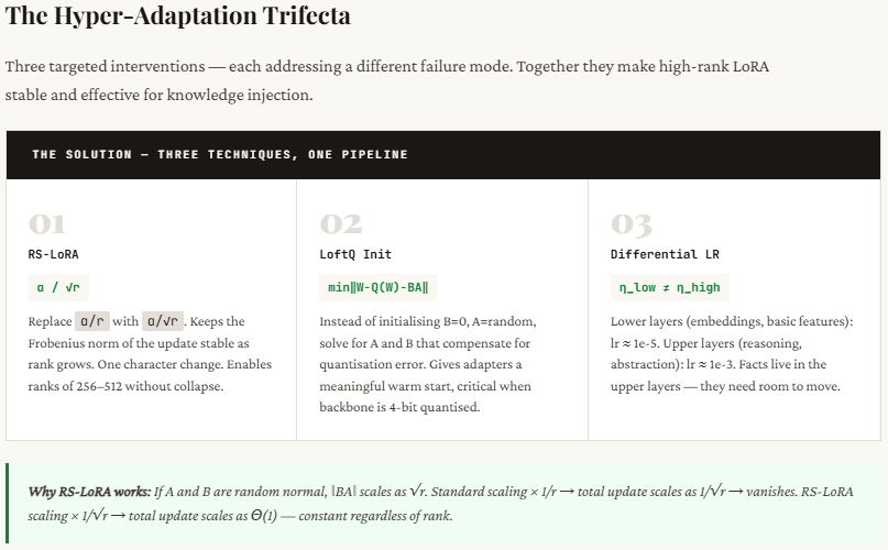
Attempting to repair this by rising the rank introduces one other drawback: instability. As rank will increase, the scaling utilized in commonplace LoRA causes the educational sign to weaken, making coaching ineffective. RS-LoRA solves this by barely adjusting the scaling formulation (altering from dividing by r to dividing by √r), which stabilizes studying even at greater ranks. This small change permits the mannequin to higher retain complicated, high-dimensional info with out breaking coaching.
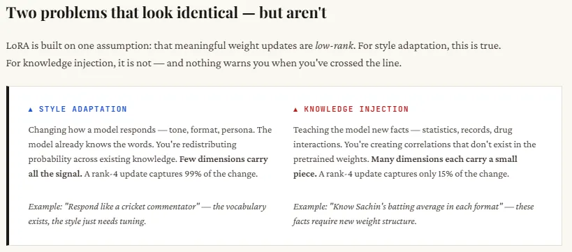
Within the code walkthrough beneath, we exhibit this failure from first rules utilizing NumPy — no coaching loops, no frameworks. We simulate two varieties of weight updates, measure precisely how a lot info survives at every rank, and expose the secondary failure: that naively rising the rank to compensate triggers a scaling collapse that kills the educational sign solely. We then present the repair — RS-LoRA’s rank-stabilized scaling — and why a single character change within the denominator (r → √r) is what makes high-rank adaptation secure.

import numpy as np
import matplotlib.pyplot as plt
import matplotlib.gridspec as gridspec

np.random.seed(42)
On this setup, we’re simulating how fine-tuning impacts a mannequin’s weight matrix by making a simplified surroundings. We assume a pre-trained weight matrix of measurement 64×64 and introduce two varieties of updates: low-rank “style” modifications (like tone or formatting) and high-rank “fact” modifications (like detailed cricket statistics). We then outline two LoRA configurations — a small rank (r=4), which represents typical LoRA utilization, and a bigger rank (r=32), which is extra appropriate for capturing complicated info as in RS-LoRA. This enables us to check how effectively completely different ranks can recuperate these simulated updates and spotlight the place commonplace LoRA struggles.
d, okay = 64, 64          # weight matrix dimensions
r_low  = 4             # LoRA rank -- small (commonplace selection)
r_high = 32            # LoRA rank -- massive (RS-LoRA suitable)

print(f"Weight matrix shape : ({d} x {k})")
print(f"Low  rank (standard): r = {r_low}")
print(f"High rank (RS-LoRA) : r = {r_high}")
print(f"Max possible rank   : {min(d, k)}")
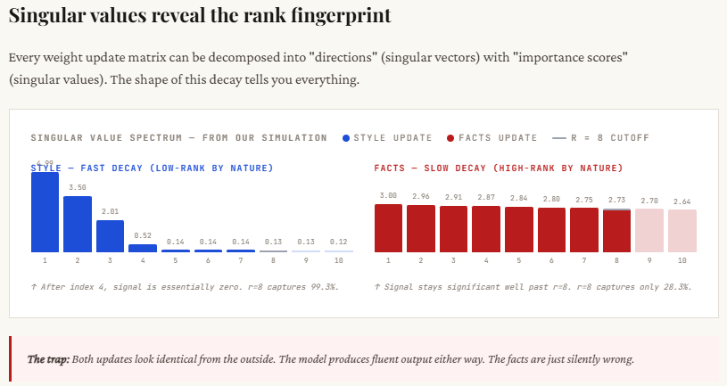
Right here, we simulate the 2 essentially several types of fine-tuning updates. The type replace is deliberately constructed as low-rank: only some singular values are massive and the remaining drop off rapidly, which means many of the vital info is concentrated in only a handful of dimensions. This mirrors real-world habits the place tone or formatting modifications don’t require widespread modification of the mannequin.
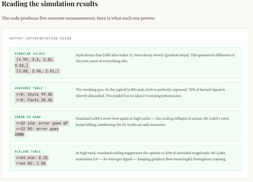
In distinction, the actual fact replace is high-rank: the singular values decay slowly, indicating that many dimensions contribute significant info. This displays how factual data (like statistics or area knowledge) is distributed throughout the mannequin. The printed singular values make this clear — type updates present a pointy drop after the primary few values, whereas reality updates stay persistently massive throughout many dimensions, proving they can’t be simply compressed right into a low-rank approximation.
def make_low_rank_delta(d, okay, true_rank, noise=0.01):
    """Simulates a style update -- low intrinsic rank."""
    U = np.random.randn(d, true_rank)
    S = np.linspace(5, 0.5, true_rank)   # fast-decaying singular values
    V = np.random.randn(okay, true_rank)
    U, _ = np.linalg.qr(U)
    V, _ = np.linalg.qr(V)
    delta = (U[:, :true_rank] * S) @ V[:, :true_rank].T
    delta += noise * np.random.randn(d, okay)
    return delta

def make_high_rank_delta(d, okay, noise=0.01):
    """Simulates a fact/knowledge update -- high intrinsic rank."""
    U = np.random.randn(d, d)
    S = np.linspace(3, 0.5, min(d, okay))   # slow-decaying -- many dimensions matter
    V = np.random.randn(okay, okay)
    U, _ = np.linalg.qr(U)
    V, _ = np.linalg.qr(V)
    delta = (U[:, :min(d,k)] * S) @ V[:, :min(d,k)].T
    delta += noise * np.random.randn(d, okay)
    return delta

delta_style = make_low_rank_delta(d, okay, true_rank=4)
delta_facts = make_high_rank_delta(d, okay)

print("nStyle  update -- top 10 singular values:", np.linalg.svd(delta_style, compute_uv=False)[:10].spherical(2))
print("Facts  update -- top 10 singular values:", np.linalg.svd(delta_facts,  compute_uv=False)[:10].spherical(2))
print("nNotice: Style decays fast → low-rank. Facts decay slowly → high-rank.")
This half compares how effectively commonplace LoRA and RS-LoRA can reconstruct the unique updates utilizing completely different ranks. Each strategies first use SVD to get the absolute best rank-r approximation (i.e., compress the replace into r dimensions), however they differ in how they scale the end result: commonplace LoRA divides by r, whereas RS-LoRA divides by √r. The desk reveals the reconstruction error — decrease means higher.
The important thing takeaway is evident: for type updates, even small ranks (like 4 or 8) work effectively as a result of the knowledge is of course low-rank, so the error rapidly drops. However for reality updates, the error stays excessive at low ranks, proving that vital info is being misplaced. Rising the rank helps, however commonplace LoRA turns into unstable because of over-scaling (error doesn’t persistently enhance). RS-LoRA, with its √r scaling, handles greater ranks extra gracefully and reduces error extra steadily, making it higher fitted to capturing complicated, high-dimensional data.
def lora_approx_standard(delta, r, alpha=16):
    """Approximate delta using rank-r LoRA with standard alpha/r scaling."""
    U, S, Vt = np.linalg.svd(delta, full_matrices=False)
    # Truncate to rank r
    B = U[:, :r] * S[:r]          # form (d, r)
    A = Vt[:r, :]                  # form (r, okay)
    scaling = alpha / r
    delta_approx = scaling * (B @ A)
    error = np.linalg.norm(delta - delta_approx, 'fro') / np.linalg.norm(delta, 'fro')
    return delta_approx, error

def lora_approx_rslora(delta, r, alpha=16):
    """Approximate delta using rank-r LoRA with RS-LoRA sqrt(r) scaling."""
    U, S, Vt = np.linalg.svd(delta, full_matrices=False)
    B = U[:, :r] * S[:r]
    A = Vt[:r, :]
    scaling = alpha / np.sqrt(r)   # <-- the important thing change
    delta_approx = scaling * (B @ A)
    error = np.linalg.norm(delta - delta_approx, 'fro') / np.linalg.norm(delta, 'fro')
    return delta_approx, error

ranks = [2, 4, 8, 16, 32, 48]

style_errors_standard, facts_errors_standard = [], []
style_errors_rslora,   facts_errors_rslora   = [], []

for r in ranks:
    _, e = lora_approx_standard(delta_style, r);  style_errors_standard.append(e)
    _, e = lora_approx_standard(delta_facts, r);  facts_errors_standard.append(e)
    _, e = lora_approx_rslora(delta_style, r);    style_errors_rslora.append(e)
    _, e = lora_approx_rslora(delta_facts, r);    facts_errors_rslora.append(e)

print("Rank | Style Err (std) | Facts Err (std) | Facts Err (RS-LoRA)")
print("-" * 60)
for i, r in enumerate(ranks):
    print(f"  {r:2d} |      {style_errors_standard[i]:.3f}      |      {facts_errors_standard[i]:.3f}      |      {facts_errors_rslora[i]:.3f}")
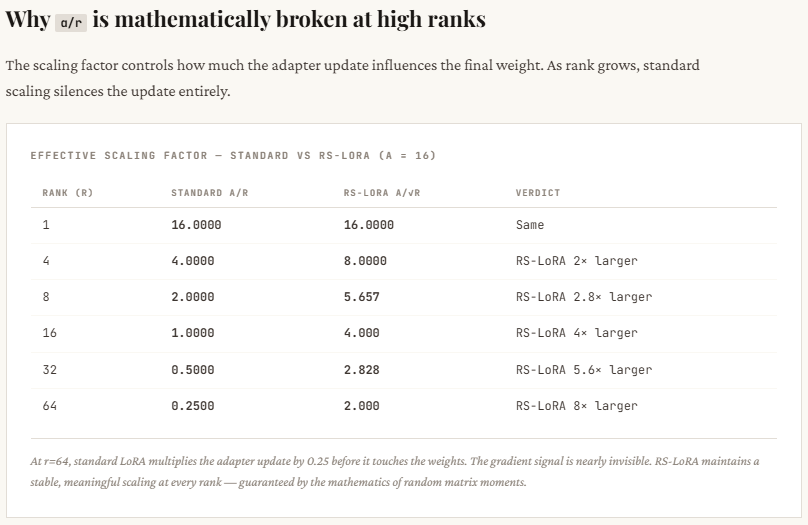
This part explains why commonplace LoRA struggles at greater ranks. Because the rank r will increase, commonplace LoRA scales the replace by α / r, which shrinks quickly — you’ll be able to see it drop from 16 (at r=1) to simply 0.25 (at r=64). Which means though you’re including extra dimensions (attempting to seize extra info), the general replace will get weaker and weaker, successfully suppressing the educational sign. The optimizer then has to compensate by pushing weights more durable, which frequently results in instability or poor convergence.
RS-LoRA fixes this by altering the scaling to α / √r. As a substitute of shrinking too aggressively, the size decreases extra regularly — staying robust sufficient even at greater ranks (e.g., nonetheless 2.0 at r=64). This retains the efficient replace magnitude significant, permitting the mannequin to really profit from higher-rank representations with out killing the sign. In easy phrases: commonplace LoRA provides capability however kills its impression, whereas RS-LoRA preserves each.
alpha = 16
rs = np.arange(1, 65)
standard_scale = alpha / rs
rslora_scale   = alpha / np.sqrt(rs)

print("nRank | Standard Scale (alpha/r) | RS-LoRA Scale (alpha/sqrt(r))")
print("-" * 55)
for r in [1, 4, 8, 16, 32, 64]:
    print(f"  {r:2d} |         {alpha/r:.4f}          |         {alpha/np.sqrt(r):.4f}")

print("nStandard scaling vanishes as rank grows.")
print("RS-LoRA scaling stays meaningful at high ranks.")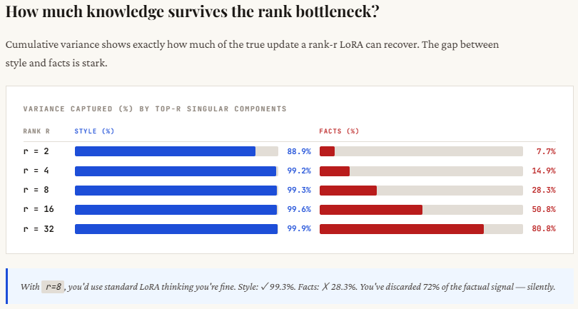
This part reveals the core distinction in how info is distributed between type and factual updates. For type, many of the vital sign is concentrated in only a few dimensions — you’ll be able to see that with rank 4, over 99% of the knowledge is already captured. For this reason low-rank strategies like LoRA work so effectively for tone, format, or persona modifications. There’s a transparent “elbow” within the singular values — after a couple of parts, the remaining don’t matter a lot.
For details, it’s the other. The data is unfold out throughout many dimensions — even at rank 8, you’re solely capturing about 28% of the whole sign, which suggests many of the data remains to be lacking. That is the “long tail” drawback: every further dimension contributes one thing vital. When LoRA truncates to a low rank, it cuts off this tail, resulting in incomplete or incorrect data. That’s why the mannequin might sound assured however nonetheless get factual particulars improper.
sv_style = np.linalg.svd(delta_style, compute_uv=False)
sv_facts  = np.linalg.svd(delta_facts,  compute_uv=False)

print("Cumulative variance captured by top-r components:n")
print(f"{'Rank':>5} | {'Style (%)':>10} | {'Facts (%)':>10}")
print("-" * 32)
total_style = np.sum(sv_style**2)
total_facts  = np.sum(sv_facts**2)
for r in [2, 4, 8, 16, 32]:
    cs = 100 * np.sum(sv_style[:r]**2) / total_style
    cf = 100 * np.sum(sv_facts[:r]**2)  / total_facts
    print(f"  {r:3d} | {cs:9.1f}% | {cf:9.1f}%")

print("nWith r=8, style is nearly fully captured.")
print("With r=8, facts are still poorly captured -- the tail matters!")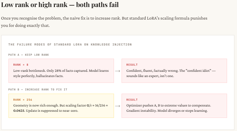
Try the Full Codes right here. Discover 100s of ML/Knowledge Science Colab Notebooks right here. Additionally, be happy to observe us on Twitter and don’t neglect to affix our 130k+ ML SubReddit and Subscribe to our E-newsletter. Wait! are you on telegram? now you’ll be able to be a part of us on telegram as effectively.
Must associate with us for selling your GitHub Repo OR Hugging Face Web page OR Product Launch OR Webinar and many others.? Join with us

I’m a Civil Engineering Graduate (2022) from Jamia Millia Islamia, New Delhi, and I’ve a eager curiosity in Knowledge Science, particularly Neural Networks and their software in varied areas.
