Sakana AI’s DiffusionBlocks: Transforming Residual Networks into Independently Trainable Denoising Modules

Scientists at Sakana AI and the University of Tokyo have introduced DiffusionBlocks, a new training framework that builds neural networks one piece at a time. Unlike conventional methods that process the entire model simultaneously, this approach cuts training memory usage by a factor of B — where B represents the total number of blocks — while delivering comparable results across a wide range of model designs.

Why Memory Becomes a Bottleneck During Training

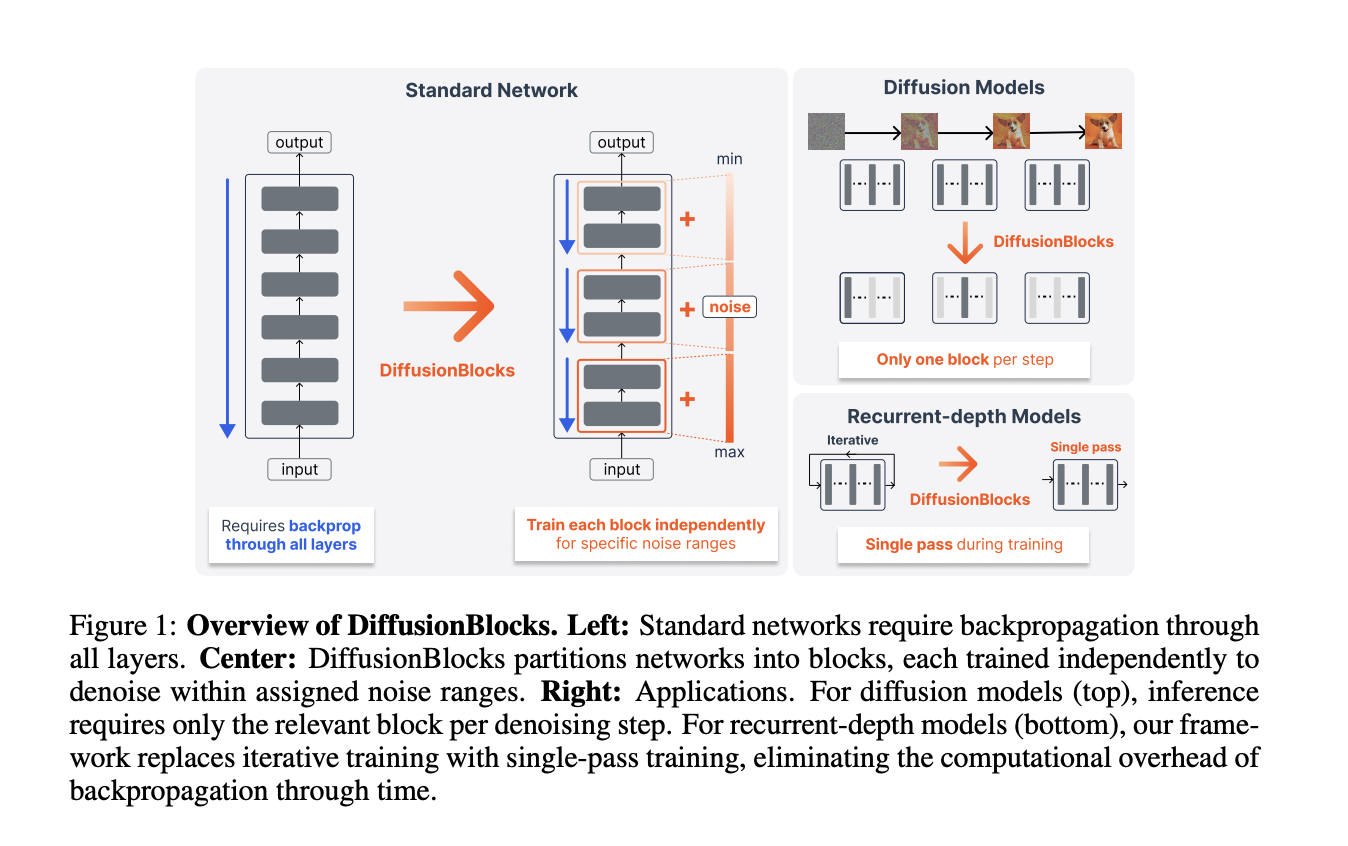
Standard end-to-end backpropagation works by saving every intermediate activation across all layers during a forward pass. Because memory needs increase in direct proportion to the number of layers, this quickly becomes a serious limitation as architectures grow deeper and more complex.

A commonly used workaround, called activation checkpointing, alleviates some of this burden by discarding certain activations and recomputing them later when needed. However, this technique does nothing to reduce memory tied up by model parameters, gradients, or optimizer states. When using the Adam optimizer, each layer must hold space for its own parameters, their gradients, and two optimizer states (one for momentum and one for variance). That adds up to four times the parameter count per layer — a figure that activation checkpointing leaves untouched.

An alternative strategy, block-wise training, takes a different path. By splitting a full network into B separate blocks and training them independently, memory requirements drop to roughly 1/B of the original. The improvement scales directly with how many blocks are used. The main difficulty, though, lies in crafting a meaningful local training objective for each individual block — one that still adds up to a well-coordinated, high-performing whole.

Earlier methods such as Hinton’s Forward-Forward algorithm and greedy layer-wise training depend on handcrafted local objectives. These approaches have consistently fallen short of end-to-end training performance and remain mostly confined to classification problems.

DiffusionBlocks fills both the theoretical void and the practical limitations that have held back previous techniques.

The Core Insight: Residual Connections as Euler Steps

The foundational idea builds on a well-known observation from prior research. In a residual network, each layer transforms its input according to $zℓ = zℓ−1 + fθℓ (zℓ−1)$. Mathematically, this mirrors the Euler discretization of an ordinary differential equation.

The research team demonstrates that these layer updates map precisely onto the probability flow ODE found in score-based diffusion models. Under the Variance Exploding (VE) formulation, the reverse diffusion process is governed by:

$frac{mathrm{d}mathbf{z}_sigma}{mathrm{d}sigma} = -sigma nabla_{mathbf{z}} log p_sigma(mathbf{z}_sigma)$

Discretizing this equation with the Euler method yields an update rule whose structure is identical to the residual connection formula. Viewed through this lens, a sequence of stacked residual blocks functions like a series of denoising operations — each one tackling a progressively different noise intensity within a defined range of [𝞂min, 𝞂max].

In score-based diffusion

Because each block learns to predict the score matching objective at its specific noise level, the training can be run separately at every noise level. In practice, each block is trained on its own using only its own local loss. There is no need for any communication between blocks while training.

Converting a Network: Three Steps

To turn a standard residual network into DiffusionBlocks, you need to make three changes:

• Block splitting: Divide the network with L total layers into B sections. Each section is a contiguous group of layers.
• Assigning noise ranges: Pick a noise distribution p_noise and set a noise range [σmin, σmax]. Split this range into B sections and give one to each block. The researchers suggest using a log-normal distribution for p_noise.
• Adding noise conditioning: Expand each block’s input so it gets a noisy copy of the target. Use AdaLN (Adaptive Layer Normalization) to tell each block what noise level it is working with. Each block then learns to recover the clean target from its noisy version within the noise range it was assigned.

During each training step, only one block is sampled and run. The rest are skipped. Memory use scales with L/B layers instead of all L layers.

Equi-probability Partitioning

A simple uniform split cuts [σmin, σmax] into equal pieces. But this misses the fact that denoising is harder at some noise levels than others. Most of the improvement in generation quality comes from intermediate noise levels when trained with a log-normal distribution.

DiffusionBlocks instead uses equi-probability partitioning. The boundaries are chosen so that each block covers exactly 1/B of the total probability under p_noise. Blocks handling intermediate noise levels get narrower intervals, while blocks at extreme noise levels get wider ones.

In tests on CIFAR-10 using DiT-S/2 with block overlap disabled to test each component separately, equi-probability partitioning reached an FID of 38.03 compared to 43.53 for uniform partitioning (lower is better). Both setups used an even layer split of [4,4,4] across 3 blocks.

Experimental Results

The team tested DiffusionBlocks on five different network types across three types of tasks. All results compare DiffusionBlocks (trained in blocks) against the same network trained end-to-end with backpropagation.

Forward-Forward comparison: On CIFAR-100, the Forward-Forward algorithm managed only 7.85% accuracy with the same ViT setup. This shows the big difference between improvised contrastive objectives and the score matching objective behind DiffusionBlocks.

Faster DiT inference: For diffusion models, each denoising step only needs one block. A 12-layer DiT with B=3 runs just 4 layers per step. This cuts inference compute by 3x compared to running all 12 layers every time.

Training Huginn models: Huginn reuses the same 4-layer block many times in a loop with stochastic recurrence, averaging 32 passes. Training uses 8-step truncated backpropagation through time (BPTT). DiffusionBlocks swaps this for a single forward pass per training step. The multi-step inference is kept as-is. Even though DiffusionBlocks trains for 15 epochs versus Huginn’s 5 epochs, the 32x reduction in steps leads to roughly 10x less total compute.

OpenWebText results: On OpenWebText, DiffusionBlocks scored 0.82 on MAUVE versus 0.85 for the baseline. Generative perplexity measured with Llama-2 was 14.99 versus 15.05. Performance was mixed, with some scores slightly below the baseline.

Handling masked diffusion: For masked diffusion models, blocks are split based on the masking schedule instead of noise levels. Each block gets an equal drop in the unmasking probability alpha(t), which keeps the parameter workload balanced across blocks.

Comparison with NoProp

NoProp is a related method that also uses a diffusion setup to train without backpropagation. It has only been tested on classification tasks with a custom CNN architecture, and no guidelines are given for applying it to other models or tasks.

DiffusionBlocks is the only approach that combines continuous-time modeling with block-wise training, and stays within 1% of the end-to-end backpropagation baseline.

Strengths and Weaknesses

Strengths:

• Built on solid theory through score matching rather than fast-hand local objectives
• Applies to five different network types without task-specific changes
• Training memory scales by a factor of B, where B is the number of blocks
• For diffusion models, inference compute also drops by B× during generation
• Equi-probability partitioning clearly beats uniform partitioning (FID 38.03 vs 43.53 on CIFAR-10)
• Eliminates the need for multi-step BPTT in recurrent-depth models, using just one forward pass
• Blocks can
  • Can be trained in parallel across GPUs without any communication overhead
  • Using a small number of blocks (B=2 or B=3) can sometimes yield better FID scores compared to training the entire network end-to-end

  Weaknesses:

  • Input and output dimensions must match; the method does not yet work with U-Net-style architectures where dimensions change across the network
  • Only tested on models trained from scratch; whether it works when fine-tuning models that were pretrained in the usual way remains unclear
  • No systematic rule exists for choosing the best number of blocks for a given model architecture and task
  • Noise conditioning introduces extra computation: the combined wall-clock training time rises to 0.0543 seconds compared to 0.0507 seconds for standard training
  • On the OpenWebText dataset, certain performance metrics fall slightly behind the standard autoregressive baseline

  Marktechpost’s Visual Explainer

  DiffusionBlocks · Sakana AI

  ICLR 2026 · Block-wise Training

  01 / 10

  A Quick Guide

  ---

  Researchers from Sakana AI and the University of Tokyo introduce DiffusionBlocks, a method that slices transformer-based networks into separate blocks, each of which can be trained on its own. Training memory drops by a factor of B, where B is the number of blocks.

  • Every block learns independently using a score matching objective grounded in continuous-time diffusion theory
  • Transformer residual connections are equivalent to Euler steps in the reverse diffusion process
  • The approach is validated on ViT, DiT, masked diffusion, autoregressive, and recurrent-depth transformers
  • For diffusion models, only one single block runs at each denoising step during inference

  02 / 10

  The Problem

  Memory Scales in Direct Proportion to Network Depth

  ---

  End-to-end backpropagation demands that intermediate activations be stored for every layer simultaneously. As networks get deeper, the memory required rises accordingly.

  Activation checkpointing lowers activation memory by recomputing values as needed during the backward pass. However, it leaves the memory required for parameters, gradients, and optimizer states untouched.

  Adam allocates extra storage per layer for parameters, gradients, and two optimizer states (first and second moments), which together come to about 4× the raw parameter memory for each layer.

  O(L)

  Activation memory required by standard end-to-end backprop

  4P

  Per-layer memory for parameters, gradients, and optimizer states when using Adam

  O(L/B)

  Memory used during DiffusionBlocks training

  03 / 10

  The Core Idea

  Residual Connections Act as Euler Steps of Reverse Diffusion

  ---

  In a residual network, each layer refines its input via z_l = z_{l-1} + f_tl(z_{l-1}). Mathematically, this is nothing other than the Euler discretization of an ordinary differential equation.

  The authors prove that these layer-to-layer updates are identical to the probability flow ODE in score-based diffusion models, under the Variance Exploding (VE) formulation.

  dz_sigma / d_sigma = -sigma · grad_z log p_sigma(z_sigma)

  This means a sequence of stacked residual blocks can be read as a series of discrete denoising steps. Since the score matching loss can be optimized separately at each noise level, every block can be trained in isolation from the others.

  04 / 10

  Conversion Recipe

  Three Adjustments to Turn Any Residual Network into DiffusionBlocks

  ---

  Step 01

  Block Partitioning

  Divide the full L-layer network into B consecutive blocks, each containing a contiguous chunk of layers.

  Step 02

  Noise Range Assignment

  Pick a log-normal distribution over noise levels and carve its range into B intervals. Each block gets one interval.

  Step 03

  Noise Conditioning

  Augment each block’s input with a noisy copy of the target signal, and inject the noise level into the block via AdaLN conditioning.

  At every training iteration, only a single block is selected and evaluated. The remaining blocks are not touched. This means the memory used equals that of L/B layers, reduced from L.

  05 / 10

  Partitioning Strategy

  Equi-Probability Intervals, Not Uniform Ones

  ---

  A straightforward uniform split divides the noise range into equal-width intervals, but this overlooks the fact that mid-range noise levels have the biggest impact on the quality of generated outputs.

  DiffusionBlocks instead picks interval boundaries so that each block takes responsibility for exactly 1/B of the total probability under the log-normal training distribution.

  Partition Strategy	Layer Distribution	FID (CIFAR-10)
  Uniform	[4, 4, 4]	43.53
  Equi-Probability	[4, 4, 4]	38.03

  Ablation study on DiT-S/2 with block overlap turned off. Lower FID values indicate better results.

  06 / 10

  Experimental Results

  Evaluated Across Five Architectures Spanning Three Types of Tasks

  ---

  Architecture	Dataset	Metric	Baseline	DiffusionBlocks	Memory
  ViT, 12L, B=3	CIFAR-100	Accuracy ↑	60.25%	59.30%	3×
  DiT-S/2, 12L, B=3	CIFAR-10	FID test ↓	39.83	37.20	3×
  DiT-L/2, 24L, B=3	ImageNet 256	FID test ↓	12.09	10.63	3×
  MDM, 12L, B=3	text8	BPC ↓	1.56	1.45	3×
  AR Transformer, B=4	LM1B	MAUVE ↑	0.50	0.71	4×
  AR Transformer, B=4	OpenWebText	MAUVE ↑	0.85	0.82	4×

  07 / 10

  Recurrent-Depth Models

  Huginn: Replacing K-Step BPTT with a Single Forward Pass

  ---

  Huginn uses a 4-layer recurrent block whose stochastic recurrence depth averages 32 iterations during training. Under conventional training, this requires 8-step truncated backpropagation through time (BPTT) to approximate the gradient.

  With DiffusionBlocks, each training step consists of just one forward pass. The multi-iteration inference procedure at test time stays exactly the same.

  0.70

  MAUVE on LM1B (compared to 0.49 baseline)

  16.08

  Perplexity under Llama-2 (compared to 17.04 baseline)

  ~10x

  Less total training compute

  08 / 10

  Comparison with NoProp

  The Sole Continuous-Time, Block-Wise Approach in the Study

  ---

  Method	Continuous-Time	Block-Wise	CIFAR-100 Accuracy
  Backpropagation	No	No	47.80%
  NoProp-DT	No	Yes	46.06%
  NoProp-CT	Yes	No	21.31%
  NoProp-FM	Yes	No	37.57%
  DiffusionBlocks	Yes	Yes	46.88%

  Evaluated using NoProp’s custom CNN architecture to ensure a fair benchmark.

  09 / 10

  Trade-offs

  Advantages and Current Drawbacks

  ---

  Advantages

  • Strong theoretical foundation via score matching, avoiding arbitrary local objectives
  • Training memory drops by a factor of B×, where B is the number of blocks
  • Unmodified compatibility with five distinct neural architectures
  • For diffusion models, inference costs are also cut by B×
  • In recurrent-depth models, it eliminates the need for K-step BPTT, replacing it with one forward pass
  • Blocks can be trained simultaneously with no communication needed between them

  Drawbacks

  • Requires input and output dimensions to match, so it can’t be used with U-Net
  • Only tested on models built from scratch, not through fine-tuning
  • No formal method yet to determine the ideal number of blocks
  • Extra wall-clock time is needed for noise conditioning
  • On OpenWebText, performance metrics slightly underperform the baseline

  10 / 10

  Read More

  Paper, Code, and Project Page

  ---

  Introduced at ICLR 2026 by Makoto Shing, Masanori Koyama, and Takuya Akiba. All code and experimental setups are publicly accessible.

  ← Previous

  01 / 10
  Next →