



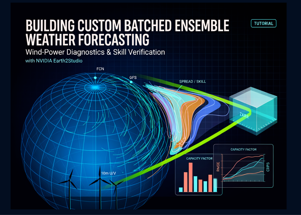
# Building Ensemble Weather Forecasts with NVIDIA Earth2Studio: A Complete Guide
## Introduction
Modern weather forecasting increasingly relies on ensemble methods to capture uncertainty across multiple possible atmospheric futures. NVIDIA Earth2Studio provides a powerful framework for building these ensemble workflows, combining deep-learning-based prognostic models with observational data sources and a rich ecosystem of diagnostics, perturbation strategies, and verification tools.
In this article, we walk through constructing a full ensemble forecasting pipeline from scratch. We cover environment setup, model loading, data ingestion, perturbation design, custom diagnostics, coordinate-aware data storage, statistical verification, and rich visualization — all within a single unified workflow.
—
## 1. Environment Setup and Dependencies
The first step involves installing Earth2Studio while carefully preserving any pre-existing CUDA-enabled PyTorch and NumPy environment. This is critical in shared computing environments such as cloud notebooks, where upgrading core libraries can break compatibility. The approach involves:
– Detecting the installed PyTorch and NumPy versions
– Writing those versions into a constraints file
– Installing Earth2Studio with the required extras (`fcn`, `data`, `perturbation`, `statistics`) while enforcing the constraints
Once installed, we configure a local cache directory for Earth2Studio, create an output folder for results, and import all necessary modules — from data retrieval and model inference to statistics, coordinate manipulation, and I/O backends.
We also check whether a GPU is available, since the FCN model benefits significantly from CUDA acceleration. If only CPU is detected, the workflow remains functional but runs considerably slower.
Key configuration parameters defined at this stage include the ensemble size, batch size, forecast duration in steps, the list of atmospheric variables to save and verify, the initialization time, and the geographic point of interest for targeted diagnostics.
—
## 2. Loading the Prognostic Model and Initial Conditions
The core forecasting engine is the FCN (Forecast Convolutional Network) model, a deep-learning architecture trained to predict the evolution of atmospheric fields. We load a pretrained FCN package and move it to the available compute device.
The model’s input and output coordinate systems define which atmospheric variables it consumes and produces, along with their spatial and temporal dimensions. From this, we determine the grid resolution (latitude and longitude arrays) that will be used throughout the workflow.
Initial conditions are retrieved from the GFS (Global Forecast System) data source, which provides gridded atmospheric analyses. The `fetch_data` utility handles downloading and preprocessing these fields, returning them as PyTorch tensors with accompanying coordinate metadata. This initial state serves as the starting point for all ensemble members.
—
## 3. Custom Wind-Power Capacity Factor Diagnostic
A valuable addition to any weather ensemble is the ability to translate raw atmospheric variables into domain-specific metrics. We implement a diagnostic model that converts 10-meter wind components (u and v) into turbine capacity factors — a measure of wind farm output normalized between 0 and 1.
The diagnostic operates in several steps:
1. **Wind speed at 10 meters** is computed from the vector magnitude of the u and v components.
2. **Hub-height wind speed** is estimated using a power-law shear relationship, scaling the 10-meter wind by the ratio of hub height to reference height raised to a specified exponent.
3. **A piecewise power curve** maps hub-height wind speed to capacity factor: below cut-in speed the output is zero, between cut-in and rated speed the output ramps cubically, above rated speed up to cut-out the output is at full capacity, and above cut-out it returns to zero.
The model integrates with Earth2Studio’s coordinate system through `input_coords` and `output_coords` methods, ensuring dimensional compatibility with upstream components. Decorators handle batched inputs automatically.
—
## 4. Variable-Scaled Perturbation System
Ensemble forecasting requires generating multiple plausible atmospheric states from a single initial analysis. Our perturbation system applies spatially correlated noise to each atmospheric variable, with amplitudes tuned to reflect the physical characteristics of each variable:
| Variable | Perturbation Amplitude |
|———-|———————-|
| Temperature at 2m (t2m) | 0.20 K |
| Temperature at 850hPa (t850) | 0.20 K |
| Geopotential height at 500hPa (z500) | 40.0 gpm |
| Geopotential height at 850hPa (z850) | 25.0 gpm |
| U-wind at 10m (u10m) | 0.25 m/s |
| V-wind at 10m (v10m) | 0.25 m/s |
| U-wind at 500hPa (u500) | 0.40 m/s |
| V-wind at 500hPa (v500) | 0.40 m/s |
| Total column water vapor (tcwv) | 0.30 kg/m² |
A critical design choice is the **control member**: ensemble member zero receives no perturbation, preserving the original deterministic forecast. This allows direct comparison between the unperturbed baseline and the spread of the ensemble, providing insight into how perturbations influence forecast outcomes.
The perturbation sampler uses either a SphericalGaussian or Brown noise process to generate spatially coherent noise fields across the global grid.
—
## 5. Building the Ensemble Execution Pipeline
The ensemble pipeline is constructed using Earth2Studio’s low-level APIs, giving full control over every stage of the forecast lifecycle:
### Data Writing Helper
A utility function selects specific atmospheric channels from multi-variable tensors and writes them into a Zarr backend — a coordinate-aware, chunked storage format optimized for array-oriented scientific data.
### Batched Ensemble Loop
The main execution function orchestrates the following sequence for each batch of ensemble members:
1. **Fetch initial conditions** from GFS for the specified initialization time
2. **Repeat** the initial state tensor across the batch size
3. **Apply perturbations** to generate distinct member states (preserving member zero as the control)
4. **Align coordinates** using Earth2Studio’s coordinate-mapping utilities to ensure compatibility with the model’s expected input format
5. **Iterate the prognostic model** step by step using the low-level `create_iterator` interface
6. **Write forecast fields** (temperature, geopotential height, wind components, water vapor) to the Zarr store after each step
7. **Chain the wind-power diagnostic** by mapping model outputs to the diagnostic’s expected coordinate system, computing capacity factors, and writing results
8. **Clear GPU memory** between batches when running on CUDA
The output Zarr dataset has dimensions for ensemble member, time step, lead time, latitude, and longitude, with each variable stored as a separate data variable.
—
## 6. Verification and Forecast Evaluation
Once forecasts are generated, rigorous verification against GFS analyses (which serve as the reference truth at forecast-valid times) quantifies accuracy and calibration. We compute four key metrics for each verification variable:
– **Latitude-weighted RMSE**: Root-mean-square error averaged over the globe with cosine-of-latitude weights to account for the convergence of meridians toward the poles.
– **Ensemble Spread**: The standard deviation of ensemble members at each grid point, latitude-weighted.
– **Fair CRPS**: The Continuous Ranked Probability Score with an unbiased correction that accounts for the finite ensemble size. This metric evaluates both accuracy and dispersion.
– **Spread-to-Skill Ratio**: The ratio of ensemble spread to RMSE. Values near one indicate a well-calibrated ensemble where spread appropriately matches forecast error.
Results are printed as tables showing how each metric evolves with forecast lead time, revealing whether the ensemble maintains skill and calibration over time.
—
## 7. Visualization of Ensemble Uncertainty
Effective visualization is essential for interpreting ensemble forecasts. We generate several types of plots:
### Spatial Maps
At the final forecast lead time, we display:
– The ensemble mean 2-meter temperature
– The ensemble spread (standard deviation) of temperature
– The GFS analysis for comparison
– The mean error (ensemble mean minus analysis)
### Geopotential Height Spaghetti Plots
Contour lines of geopotential height at 5520 meters show how individual ensemble members diverge over time, with the control member highlighted in black, perturbed members in blue, and the GFS analysis in red.
### Point-Based Fan Charts
For New Delhi, we plot a fan chart of 2-meter temperature showing the ensemble range, mean trajectory, control member, and observations. A companion panel shows the wind capacity factor forecast at the same location, demonstrating how the custom diagnostic extends the value of the ensemble.
### Lead-Time Skill Curves
RMSE, spread, and fair CRPS are plotted as functions of forecast lead time for each verification variable, providing a clear picture of how forecast skill degrades and how ensemble spread evolves over the prediction horizon.
### Data Inspection
Finally, we open the complete Zarr dataset with Xarray to enable interactive exploration, subsetting, and export of the full ensemble structure.
—
## 8. Key Takeaways
This workflow demonstrates how Earth2Studio’s modular architecture enables the construction of sophisticated ensemble forecasting systems without relying on monolithic, pre-built ensemble functions. By combining component-level APIs for data, models, perturbations, diagnostics, batching, coordinate management, and I/O, users retain full flexibility to customize every aspect of the pipeline.
The ability to physically scale perturbations per variable, maintain an unperturbed control member, chain custom diagnostics, and persist results in a coordinate-aware format makes this approach both scientifically rigorous and practically extensible.
—
## Frequently Asked Questions (FAQ)
**Q1: What is Earth2Studio and what does it do?**
Earth2Studio is an NVIDIA-developed framework for building climate and weather analysis and forecasting workflows. It provides modular components for data retrieval, deep-learning-based forecasting, perturbation generation, statistical verification, and data persistence — all designed to work together seamlessly.
**Q2: Why is the FCN model used for weather forecasting?**
The FCN (Forecast Convolutional Network) is a neural-network-based prognostic model trained to predict the evolution of atmospheric fields from initial conditions. It offers fast inference compared to traditional numerical weather prediction and can capture complex nonlinear atmospheric dynamics.
**Q3: What role does GFS play in this workflow?**
GFS (Global Forecast System) serves dual purposes: it provides the initial atmospheric conditions (analyses) used to start the forecasts, and its analyses at forecast-valid times serve as the reference truth for evaluating forecast accuracy.
**Q4: Why are perturbation amplitudes different for each variable?**
Different atmospheric variables have different physical scales and sensitivities. Temperature perturbations are measured in Kelvin, wind perturbations in meters per second, and geopotential height perturbations in geopotential meters. The amplitudes are chosen to reflect realistic uncertainties in each variable.
**Q5: What is the significance of the control member?**
The control member (ensemble member zero) receives no perturbation and represents the deterministic forecast baseline. Comparing it against the spread of perturbed members helps assess how much the initial-condition uncertainty contributes to forecast divergence.
**Q6: How does the wind-power capacity factor diagnostic work?**
It takes 10-meter wind components, computes wind speed, scales to hub height using a power-law shear exponent, and maps the result through a piecewise cubic power curve that defines output as a fraction between zero (no output) and one (full capacity), depending on wind speed relative to cut-in, rated, and cut-out thresholds.
**Q7: What is fair CRPS and why is it used?**
The fair (unbiased) Continuous Ranked Probability Score corrects the standard CRPS for finite ensemble size. It provides a rigorous measure of both forecast accuracy and calibration, penalizing ensembles that are either too narrow or too wide relative to observed errors.
**Q8: Why use Zarr format for storing forecasts?**
Zarr is a chunked, coordinate-aware array format designed for efficient storage and access of large multidimensional scientific datasets. It supports parallel I/O, compression, and integrates naturally with Xarray for analysis and visualization.
**Q9: Can this workflow be extended to other models or data sources?**
Yes. Because Earth2Studio uses standardized component interfaces for models, data sources, perturbations, and diagnostics, users can swap in different prognostic models, connect alternative data providers, add new diagnostic tools, or scale the ensemble size without redesigning the pipeline.
**Q10: What hardware is recommended for running this workflow?**
A GPU (CUDA-enabled) is strongly recommended due to the computational demands of running multiple ensemble members through a deep-learning model over multiple time steps. CPU-only execution is possible but will be substantially slower.
—
## Conclusion
We have presented a complete guide to constructing an ensemble weather forecasting workflow using NVIDIA Earth2Studio. From environment configuration and model loading through custom perturbation design, diagnostic chaining, coordinate-aware data persistence, rigorous statistical verification, and multi-faceted visualization — every stage of the ensemble lifecycle is covered using Earth2Studio’s modular, composable APIs.
The resulting system produces a rich Zarr dataset containing ensemble forecasts for multiple atmospheric variables alongside derived diagnostics such as wind capacity factors. Verification metrics including latitude-weighted RMSE, fair CRPS, ensemble spread, and spread-skill ratios provide quantitative insight into forecast quality and calibration across all lead times.
Because each component adheres to Earth2Studio’s standard interfaces, the workflow is inherently extensible — new models, data sources, diagnostics, and storage backends can be integrated as drop-in replacements, enabling researchers and practitioners to iterate rapidly on ensemble forecasting experiments.
Thank you for reading
