



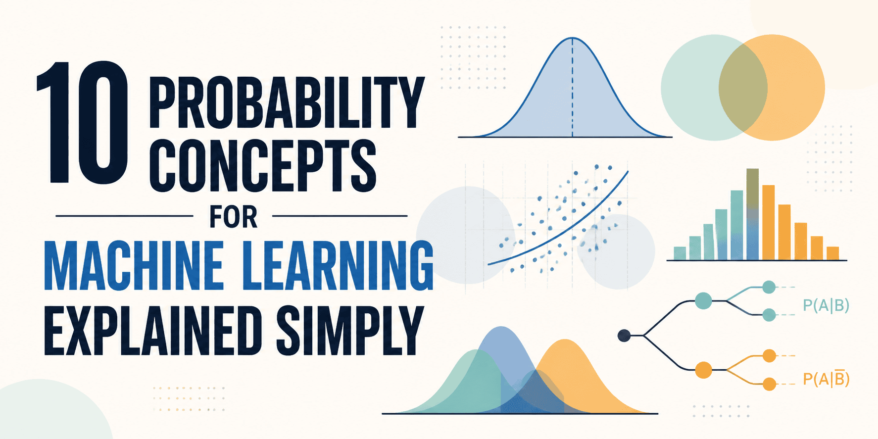
Below is a restructured, SEO-optimized article based on the full content you provided (which focuses on ten core probability concepts critical for machine learning), followed by a citation of the original source.
—
## Master Machine Learning with These 10 Probability Concepts
Probability is often treated as a prerequisite “vegetable” in machine learning—something to get through before reaching the “good part.” In reality, probability is what makes much of machine learning work. Models rarely give hard yes/no answers; instead, they express confidence in the form of probabilities. If you understand the core ideas below, probability stops feeling like memorization and starts feeling like a practical tool.
### 1. Random Variables
In machine learning, almost everything—features, labels, errors, and outputs—depends on outcomes we haven’t yet observed. Any such quantity is called a **random variable**.
– Denoted with uppercase letters like (X) or (Y)
– Observed values use lowercase letters ((x), (y))
– In supervised learning, we aim to estimate (P(Y mid X)): Given inputs (X), what is the probability of each label (Y)?
For example, a spam classifier might output (P(Y=1 mid X=x)=0.92), meaning “92% sure this email is spam.”
### 2. Probability Distributions
A probability distribution describes which values a random variable can take and how likely each value is.
– **Discrete distributions**: Probabilities sum to 1, (sum_x P(X=x)=1)
– **Continuous distributions**: Probability is described by a density where the area under the curve equals 1, (int_{-infty}^{infty} p(x),dx=1)
Common examples:
– **Bernoulli distribution** for binary events (e.g., spam or not spam)
– **Gaussian (normal) distribution** for continuous values like prediction errors
Machine learning models often learn entire distributions: classifiers estimate (p_theta(y mid x)), the probability of each class given the input.
### 3. Expectation, Variance, and Standard Deviation
– **Expectation (mean)**: The long-run average value you expect:
– Discrete: (mathbb{E}[X] = sum_x x P(X=x))
– Continuous: (mathbb{E}[X] = int x,p(x),dx)
– **Variance**: Measures how spread out values are around the mean
– **Standard deviation**: The square root of variance, preferred because it’s in the same units as the original data
Two models can have identical average errors but very different reliability—standard deviation reveals that difference.
### 4. Conditional Probability
Models almost always reason given what they observe. Conditional probability answers:
[
P(A mid B) = frac{P(A cap B)}{P(B)}
]
In classification, this is exactly what we want: (P(Y mid X)), the probability of a label given the features. For instance:
[
P(text{Spam} mid text{contains “free”}) = 0.8
]
Observing evidence (like keywords) updates our beliefs.
### 5. Bayes’ Theorem
Bayes’ theorem formalizes how to update beliefs when new evidence appears:
[
P(A mid B) = frac{P(B mid A) P(A)}{P(B)}
]
Components:
– (P(A)): prior belief before seeing evidence
– (P(B mid A)): how likely the evidence is if (A) is true
– (P(B)): overall probability of the evidence
– (P(A mid B)): updated belief after seeing evidence
This underpins Bayesian classifiers, Bayesian neural networks, and diagnostic reasoning systems.
### 6. Joint, Marginal, and Conditional Distributions
– **Joint distribution** (P(X,Y)): probability of multiple events occurring together
– **Marginal distribution**: probability of one variable alone, obtained by summing/integrating out the others
– **Conditional distribution**: probability of one event given another, expressed via the joint
Independence occurs when (P(X,Y) = P(X)P(Y)), meaning the variables provide no information about each other. Naive Bayes assumes conditional independence of features given the class label—a “lie” that works surprisingly well for text.
### 7. Likelihood and Maximum Likelihood Estimation (MLE)
Likelihood measures how probable the observed data is under a given set of model parameters. For (n) independent examples:
[
mathcal{L}(theta) = prod_{i=1}^{n} p_theta(y_i mid x_i)
]
**Maximum Likelihood Estimation** finds parameters that maximize this likelihood:
[
hat{theta}_{text{MLE}} = argmax_theta mathcal{L}(theta)
]
In practice, we maximize the log-likelihood for numerical stability, which is equivalent to minimizing cross-entropy loss used in classification tasks.
### 8. Sampling, Law of Large Numbers, and Central Limit Theorem
– **Sample mean** (bar{X}) estimates the true expected value
– **Law of Large Numbers**: As sample size grows, the sample mean converges to the true mean
– **Central Limit Theorem**: Averages of many independent samples become approximately normally distributed, with standard error (sigma/sqrt{n})
These results justify mini-batch training, A/B testing, and validation sets—core practices that rely on samples representing the whole.
### 9. Entropy, Cross-Entropy, and KL Divergence
– **Entropy** (H(p)) measures uncertainty in a distribution
– **Cross-entropy** (H(p,q)) measures how well predicted distribution (q) matches the true distribution (p)
– **KL divergence** quantifies the difference between two distributions
Lower entropy means higher confidence. Cross-entropy is the standard loss function for classification, heavily penalizing confident wrong predictions.
### 10. Calibration and Predictive Uncertainty
A model can be accurate yet poorly calibrated—overconfident in its predictions. Calibration checks whether predicted probabilities reflect true frequencies:
– A model that says “80% confidence” should be correct about 80% of the time
– The Brier Score evaluates calibration quality
Well-calibrated uncertainty is critical in high-stakes domains like healthcare, finance, and autonomous systems.
—
### Final Thoughts
Probability is not a side topic in machine learning—it explains what models are really doing under the hood. These ten concepts provide a durable foundation. Once they feel like tools rather than obstacles, the rest of machine learning becomes much clearer.
—
**Reference**
Original article excerpt: “10 Probability Concepts for Machine Learning Explained Simply.” *KDNuggets*. [https://www.kdnuggets.com/wp-content/uploads/kdn-10-probability-concepts-for-machine-learning-explained-simply.png](https://www.kdnuggets.com/wp-content/uploads/kdn-10-probability-concepts-for-machine-learning-explained-simply.png)
