



# Understanding the SIFT Algorithm: A Comprehensive Guide to Scale-Invariant Feature Detection and Matching
## Introduction
In the field of computer vision, one of the enduring challenges is recognizing the same object across images that differ in scale, orientation, lighting, and viewpoint. The Scale-Invariant Feature Transform, widely known as SIFT, was designed to address precisely this challenge. It remains one of the most influential algorithms in the domain, providing a reliable framework for detecting distinctive keypoints in images, describing them with robust feature vectors, and matching those features across different photographs of the same scene or object.
What makes SIFT particularly powerful is its dual invariance to scale and rotation. This means that whether an object appears large or small in an image, or whether it has been rotated to a different angle, SIFT can still identify and match its distinctive features with remarkable consistency. These properties have made it a cornerstone technique in applications ranging from image retrieval and object recognition to panorama creation and 3D scene reconstruction.
This guide walks through the inner workings of SIFT, from the initial construction of scale-space representations to the final comparison of feature descriptors, providing a thorough understanding of each stage in the pipeline.
—
## How SIFT Works: A Step-by-Step Breakdown
### Building a Multi-Scale Representation of the Image
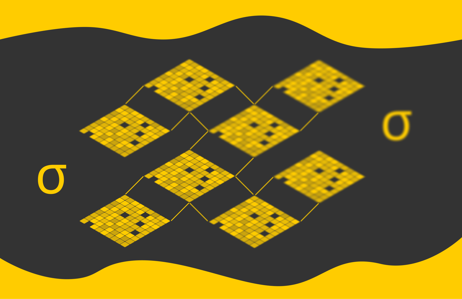
The first stage of SIFT involves creating multiple versions of the original image, each representing the scene at a different level of blur. This process allows the algorithm to detect features at various scales, from fine details to broad structural patterns.
Starting with the original image, SIFT applies Gaussian smoothing with progressively increasing standard deviations. If we denote the original image as **I(x, y)**, the algorithm generates a sequence of blurred images using values such as **σ₁, k·σ₁, k²·σ₁, k³·σ₁**, and so on, where **k > 1**. The result is a chain of images in which each successive frame is slightly more blurred than the one before it. This chain is referred to as an **octave**.
Once this sequence is constructed, SIFT computes the pixel-wise differences between adjacent blurred images. These differences, known as the **Difference of Gaussians (DoG)**, highlight regions of rapid intensity change — essentially pinpointing areas of interest such as edges, corners, and blobs.
### Detecting Keypoints via Local Extrema
With the DoG images in hand, SIFT searches for local extrema — pixels that are either the brightest or the darkest compared to their neighbors. For each pixel in a DoG layer, the algorithm examines a 3×3×3 neighborhood consisting of:
– **8 adjacent pixels** on the same DoG layer (the immediate 2D neighbors)
– **9 pixels** on the layer directly above (one scale coarser)
– **9 pixels** on the layer directly below (one scale finer)
A pixel is marked as a keypoint candidate if it is either greater than all 26 neighbors (a local maximum) or less than all 26 neighbors (a local minimum). Points that do not satisfy either condition are discarded. This three-dimensional comparison ensures that keypoints are distinctive not only in the spatial domain but also across different scales, which is critical for handling objects at varying distances and sizes.
Since the initial round of extrema detection often produces a large number of candidates — many of which correspond to noise or low-contrast regions — SIFT applies a contrast threshold to filter out weak features. Only keypoints with a sufficiently strong intensity change are retained as stable interest points.
### Why Use the Difference of Gaussians Instead of the Laplacian of Gaussian?
Historically, the Laplacian of Gaussian (LoG) has been a popular technique for edge detection and blob identification. However, computing LoG for multiple scales is computationally expensive. SIFT uses the DoG as a practical approximation to LoG, and the mathematical relationship between the two is well established:
**DoG ≈ (k − 1) · σ² · ∇²nσ**
In essence, the DoG can be thought of as a scaled version of the LoG. Because the DoG is derived from simple subtraction of two already-computed Gaussian-blurred images, it is far cheaper to compute than applying the full LoG formula repeatedly. This approximation preserves the key properties of LoG while dramatically reducing computational cost, making SIFT practical for real-world use.
### Constructing Multiple Octaves for Efficient Multi-Scale Detection
Rather than building a single sequence of increasingly blurred versions of the full-resolution image, SIFT organizes its scale-space into multiple octaves. Each octave begins with an image that has been downsampled by a factor of two in both width and height. The first octave uses the original image resolution, the second octave works on a half-resolution version, the third on a quarter-resolution version, and so on.
This multi-octave design offers two significant advantages. First, as blur increases, fine image details disappear, so there is little benefit to maintaining full resolution at coarse scales. Downsampling reduces the pixel count by a factor of four at each octave, dramatically speeding up subsequent processing. Second, very large Gaussian blur kernels introduce approximation errors, but downsampling a smaller image can mimic the effect of a larger blur on a full-resolution image without incurring those errors. Together, these benefits make octave-based processing both faster and more accurate.
### Why a Three-Dimensional Search Window?
A two-dimensional window (3×3) can find local extrema within a single blurred image, but the sheer number of candidate points across multiple scales would be overwhelming. By extending the search to three dimensions — two spatial dimensions plus the scale dimension — SIFT ensures that only the most stable and distinctive keypoints survive. Points that are local extrema only within a single scale layer but not across neighboring scales are discarded, resulting in a compact set of high-quality interest points.
### Computing SIFT Feature Descriptors
Once stable keypoints have been identified, SIFT constructs a descriptor for each one. This descriptor is what enables matching across images, as it encodes the local appearance of the image patch around the keypoint in a compact numerical form.
The process begins by mapping each detected keypoint to a circular region in the original image. The radius of this circle depends on the scale at which the keypoint was detected — higher blur levels correspond to larger circles, reflecting the fact that features detected at coarser scales encompass broader image regions.
Within each circle, SIFT computes the gradient magnitude and orientation for every pixel. The image region is then divided into four equal quadrants, and for each quadrant, a distribution of gradient directions is built. These four histograms are concatenated, normalized, and clipped to produce a final **128-dimensional feature vector**. This vector serves as the descriptor for the keypoint.
SIFT includes safeguards for situations where the circular region contains fewer than 128 pixels; in such cases, information from neighboring pixels is incorporated to still produce a full-length descriptor.
### Achieving Rotation Invariance
A common real-world scenario is when the same object appears in two images but is rotated by different amounts. To handle this, SIFT determines the **principal orientation** of each keypoint — the dominant gradient direction within its local neighborhood. This orientation is used to rotate the coordinate system before computing the descriptor, effectively aligning all instances of the same feature to a canonical orientation. This mechanism guarantees that rotated versions of the same object produce matching descriptors, contributing to SIFT’s robustness.
—
## Comparing SIFT Descriptors
After descriptors have been computed for keypoints in two images, the next step is to determine which descriptors correspond to the same physical feature. Two common metrics are used for this purpose:
– **L2-distance (Euclidean distance):** The square root of the sum of squared differences between two descriptor vectors. A lower L2-distance indicates a better match, with a distance of zero representing a perfect match.
– **Histogram intersection:** This metric compares two descriptors by summing the minimum value of each corresponding vector component. It measures how well the gradient direction distributions overlap between two features. A higher histogram intersection value signifies a stronger match.
These comparisons form the basis of feature matching, where keypoints in one image are paired with their best counterparts in another image based on descriptor similarity.
—
## Applications of SIFT
### Image Matching and Alignment
One of the most direct applications of SIFT is matching the same scene or object across two or more images. By computing descriptors for each image and comparing them, SIFT can establish correspondences even when the images differ in scale, rotation, or viewpoint. These correspondences can then be used to align images, estimate camera motion, or stitch photographs together.
### Object Detection and Recognition
Given a template image of an object, SIFT can search a larger scene for instances of that object. Keypoints detected on the template are matched against keypoints found in the scene, and the resulting set of good matches indicates the location and presence of the object. SIFT’s tolerance to partial occlusion makes it particularly useful in this context — even if parts of the object are hidden behind other structures, enough visible features can still be matched to confirm its presence.
### Image Stitching and Panorama Creation
By matching features across multiple overlapping photographs, SIFT provides the foundation for image stitching — the process of combining several images into a seamless, wide-angle panorama. Once feature correspondences are established, geometric transformations (such as homographies) can be computed to warp each image into a common coordinate frame, which is then blended into a unified result.
### 3D Scene Reconstruction
While SIFT alone does not reconstruct three-dimensional geometry, it plays a vital role in pipelines for 3D reconstruction. By matching features across many images taken from different viewpoints, SIFT provides the correspondences needed to estimate camera positions and triangulate 3D points. Algorithms such as COLMAP rely on SIFT as their primary feature extraction and matching step to build dense 3D models from image collections.
—
## FAQ
### What does SIFT stand for?
SIFT stands for **Scale-Invariant Feature Transform**. It is named for its ability to detect and describe image features in a way that is invariant to changes in scale and rotation.
### Why is SIFT considered scale-invariant?
SIFT processes the image at multiple scales by constructing Gaussian-blurred versions at different levels of blur and at different resolutions (octaves). Keypoints are detected by comparing each pixel across both spatial and scale dimensions, ensuring that features are identified consistently regardless of their size in the image.
### What is the Difference of Gaussians, and why is it used?
The Difference of Gaussians (DoG) is computed by subtracting one Gaussian-blurred image from another with a slightly different blur level. It serves as a computationally efficient approximation of the Laplacian of Gaussian (LoG), which is a well-known technique for detecting edges and blobs in images. DoG preserves the key detection properties of LoG while requiring far less computation.
### How does SIFT handle rotated objects?
SIFT computes the principal orientation of each keypoint by finding the dominant gradient direction in its local neighborhood. When constructing the feature descriptor, SIFT rotates the coordinate system so that this principal orientation aligns with a canonical direction. This ensures that descriptors are rotation-invariant.
### What is a SIFT descriptor?
A SIFT descriptor is a 128-dimensional vector that encodes the distribution of gradient orientations within the local neighborhood of a keypoint. It is constructed by dividing the region around the keypoint into four quadrants, computing a histogram of gradient directions for each, and concatenating the results. This compact representation is robust to small changes in viewpoint and illumination.
### Can SIFT work with color images?
SIFT operates on grayscale images. Color images must first be converted to grayscale before SIFT is applied. While this discards color information, the gradient-based features that SIFT computes from intensity values are generally sufficient for reliable matching.
### What are the limitations of SIFT?
SIFT can be relatively slow compared to newer algorithms, especially on high-resolution images, due to the extensive multi-scale processing required. It may also produce false-positive matches in textureless or highly repetitive regions. Additionally, SIFT is patented (though the patent has expired), which historically influenced the development of alternative algorithms such as ORB and SURF.
### How are false matches removed?
After initial matching, techniques such as **Lowe’s ratio test** compare the distance to the best match against the distance to the second-best match. If the best match is significantly closer, it is retained; otherwise, it is discarded. Additional geometric filtering methods, such as RANSAC, can further eliminate inconsistent matches by fitting a geometric model to the correspondences.
—
## Conclusion
The SIFT algorithm represents a landmark achievement in computer vision, providing a robust and elegant solution for detecting, describing, and matching image features across varying scales and orientations. Its multi-stage pipeline — from scale-space construction through DoG extrema detection to 128-dimensional descriptor generation — has influenced countless subsequent algorithms and continues to serve as a reliable backbone for a wide range of practical applications.
Whether used for aligning photographs, recognizing objects in complex scenes, creating panoramas, or enabling 3D reconstruction pipelines, SIFT’s combination of scale invariance, rotation invariance, and descriptive power has solidified its place as a foundational technique in the computer vision toolkit.
Thank you for reading
