



# Transferable Models for Predicting Retention Times in Liquid Chromatography: Advances and Applications
## Introduction
Predicting how long a compound will take to travel through a liquid chromatography (LC) system has become one of the most pursued goals in modern analytical chemistry. For researchers analyzing metabolites and other small molecules, knowing retention times in advance can dramatically accelerate identification workflows, reduce experimental costs, and improve the reliability of molecular annotations. In a typical untargeted metabolomics experiment, thousands of molecular features may be detected, yet only a fraction can be confidently identified using spectral matching alone. Retention time information offers an orthogonal dimension of evidence that can resolve ambiguities and increase confidence in compound assignments.
Recent work has demonstrated that machine learning models, particularly those based on graph neural networks and directed message-passing architectures, can learn the complex relationship between molecular structure and chromatographic behavior. However, a critical challenge remains: can a model trained on one chromatographic setup reliably predict retention times or retention orders in a completely different setting? This question of *transferability* lies at the heart of practical applicability. A model that only works for the exact column, mobile phase, and gradient conditions seen during training has limited utility in real laboratories where methods frequently change.
This article explores the design, training, and evaluation of transferable retention time models, focusing on reversed-phase liquid chromatography datasets compiled from the scientific literature. We examine how molecular representations, chromatographic parameters, and training strategies combine to produce models capable of generalizing across diverse experimental conditions.
## Data Collection and Curation
### Building a Representative Training Corpus
The foundation of any reliable predictive model is high-quality training data. Researchers compiled a large collection of reversed-phase LC datasets encompassing measurements of small molecules and metabolites. Using comprehensive literature searches, they identified over 2.3 million publications related to small molecule analysis by liquid chromatography, with approximately 2,400 of those specifically addressing retention time prediction, and roughly 2,000 dealing with quantitative structure-retention relationships.
From these publications, 297 reversed-phase datasets were initially considered for model development. Careful filtering removed datasets that were too small (fewer than 20 compounds), those with incomplete gradient coverage, those measured under suspicious or inconsistent conditions, and those using unconventional gradient types such as step-wise elution. Datasets using step-wise gradients were particularly problematic, as their retention order patterns differed substantially from the ramp gradients used in the vast majority of other datasets, with over 94% of compound pairs appearing in conflicting order on average.
### Handling Missing Chromatographic Parameters
A significant challenge in curating the training data was the incomplete availability of column characterization parameters. Parameters such as hydrophobic subtraction model (HSM) values and Tanaka parameters require specialized experiments using authentic standards under specific analytical conditions. These experiments are often incompatible with the liquid chromatography–mass spectrometry (LC–MS) setups commonly used in metabolomics studies. As a result, pH, HSM, or Tanaka parameters were missing from approximately one-third of the remaining datasets. After excluding those with insufficient parameter information, 171 datasets remained as the final training corpus, referred to as the curated training data.
### Defining Retention Order and Void Volume
Not all compounds in a chromatographic run are retained by the stationary phase. Some compounds pass through the column essentially unretained, emerging at the void volume—the combined volume of the column packing and connecting capillaries. Compounds eluting within the void volume provide little information about structure–retention relationships and were treated specially. In cases where the actual void volume of a dataset was unknown, researchers used twice the estimated value as a conservative threshold. Approximately 22% of all entries across the datasets eluted within this void volume window.
For models that predict retention order rather than absolute retention times, pairs of compounds where both elute in the void volume were excluded from training and evaluation, since no meaningful order information can be extracted from such pairs.
## Model Architecture and Training Strategy
### Directed Message-Passing Neural Networks for Retention Order
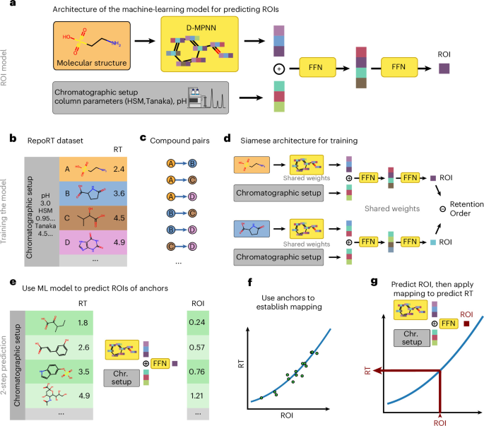
The core architecture for predicting retention order indices (ROI) uses a directed message-passing neural network (D-MPNN). This type of model processes molecular structures as graphs, where atoms serve as nodes and chemical bonds serve as edges. Through multiple rounds of message passing, each atom aggregates information from its neighbors, building up a holistic representation of the entire molecule.
The D-MPNN encoding process begins by assigning initial feature vectors to each atom and bond based on properties such as atomic number, mass, hydrogen count, charge, chirality, aromaticity, and hybridization. Three message-passing steps are then performed, updating these embeddings iteratively. The final molecular representation is obtained by averaging the atom-level embeddings, producing a fixed-size vector of 512 dimensions.
To this molecular embedding, standardized chromatographic setup parameters are appended as a 13-dimensional vector. This vector encodes the pH of the mobile phase as a single value, along with twelve stationary-phase descriptors: six HSM parameters capturing hydrophobic interaction, steric effects, hydrogen bond acidity and basicity, and cation exchange activity at two pH values, and six Tanaka parameters describing hydrophobicity, hydrophobic selectivity, steric selectivity, hydrogen bonding capacity, and ion exchange capacity at two pH values.
The combined molecule-and-system embedding is then processed through several feed-forward neural network layers, progressively distilling the information into a single scalar output—the retention order index. ReLU activation functions are used throughout the hidden layers, and the model employs approximately 951,000 learnable parameters when chromatographic features are included.
### Training with Siamese Learning and Weighted Pairs
The model is trained using a Siamese architecture, where two copies of the same network—with identical weights—simultaneously predict the retention order indices for two compounds in a pair. A margin ranking loss function then penalizes the model when the predicted order does not match the experimentally observed order, encouraging the model to learn the correct relative ranking.
Compound pairs are weighted during training based on the difference in their experimental retention times. Pairs with small retention time differences (less than 30 seconds) receive substantially lower weight, reflecting the greater uncertainty in determining which compound elutes first. Pairs separated by more than 60 seconds receive essentially full weight. This weighting scheme prevents noisy, borderline pairs from dominating the training signal.
To ensure fair treatment across datasets of varying sizes, training pairs are sampled uniformly: first a dataset is chosen at random, then a compound pair is drawn uniformly from within that dataset. Each training epoch processes 500,000 compound pairs. The Adam optimizer is used with a fixed learning rate, and training proceeds for a maximum of ten epochs—enough to achieve convergence while avoiding the overfitting that becomes apparent with longer training runs.
## Evaluating Transferability
### Challenging Dataset Splits
A standard approach to evaluating predictive models is to hold out some datasets and test performance on them. However, this naive split can be overly optimistic when models simply memorize the conditions of the held-out datasets. To truly assess transferability, researchers designed evaluation protocols that are progressively more challenging:
1. **Standard split**: No dataset in the training set shares a nominally identical chromatographic setup with any dataset in the test set.
2. **Challenging split**: Beyond avoiding identical setups, training datasets sharing the same column and a similar mobile phase pH (within one pH unit of the test dataset) are also excluded.
3. **Without target compounds**: All compounds and their stereoisomers present in the test dataset are removed from the training data.
4. **Maximum challenge**: Both similar datasets and target compounds are excluded simultaneously.
These splits mimic realistic scenarios where a laboratory might change columns, adjust mobile phase pH, or encounter entirely new compound classes not seen during model development.
### Baseline Models for Comparison
Several baseline methods were evaluated alongside the neural network approach. The RankSVM, a support vector machine adapted for ranking tasks, was tested using molecular fingerprints as compound representations. Training RankSVM on all available datasets was projected to require over one month of computation, so a subset of 100 datasets was used for benchmarking.
Another baseline, referred to as RankNet, uses classical molecular descriptors calculated by the RDKit cheminformatics toolkit. These descriptors capture features such as molecular weight, logP, polar surface area, and counts of various functional groups. A feed-forward neural network with a single hidden layer of 256 neurons was trained on these descriptors, following the same training protocol as the D-MPNN model to ensure fair comparison.
## From Retention Order to Absolute Retention Time
Predicting whether compound A elutes before or after compound B is valuable, but practical metabolomics workflows benefit even more from knowing the actual retention time in minutes. Converting a retention order index into an absolute retention time requires a calibration step using a small set of anchor compounds with known retention times.
The calibration mapping is established in two stages. First, a constrained median regression is performed using a second-degree polynomial, with coefficients restricted to be non-negative to enforce a monotonically increasing relationship between ROI and retention time. Anchor compounds with errors exceeding twice the median error are then discarded as potential outliers. A refined mapping is computed using ordinary least squares regression, and if the resulting function is not monotonically increasing, the earlier median regression result is retained instead.
Several robust fitting alternatives were also compared, including generalized additive models (GAM), smooth additive models (SCAM), and constrained oblique basis splines (COBS). All of these enforce monotonicity, ensuring that the mapping preserves the fundamental property that stronger retention corresponds to longer retention times.
## Direct Retention Time Prediction Models
### DeepGCN-RT and RT-Transformer
Beyond the two-step approach of first predicting retention order and then calibrating to absolute times, direct retention time prediction models were also evaluated. DeepGCN-RT uses a deep graph convolutional network architecture, while RT-Transformer employs a transformer-based attention mechanism. Both follow a pre-training and fine-tuning paradigm.
For pre-training, models were exposed to either a large homogeneous dataset called SMRT or the diverse RepoRT repository. The RepoRT repository, spanning many different experimental setups and compound classes, more closely resembles the distribution of biomolecules commonly encountered in metabolomics studies. Two pre-training strategies were compared: a single pre-training pass concatenating all datasets, and a repeated pre-training approach where the model was sequentially trained on individual datasets, carrying forward learned weights between them.
For fine-tuning, six frequently used benchmark datasets were employed, with compounds in the void volume, duplicates, and doublets carefully removed. The curated versions of these datasets, with standardized molecular representations, ensured consistent evaluation conditions.
## Real-World Application: Fecal Metabolomics
### Predicting Retention Times for Unknown Metabolites
To demonstrate the practical impact of transferable retention time prediction, a public human fecal metabolomics dataset was analyzed. The study involved extracting metabolites from fecal samples using standardized protocols, separating them on a C18 reversed-phase column, and detecting them with high-resolution mass spectrometry.
Using a trained retention order prediction model and a small set of 19 N-alkylpyridinium 3-sulfonate (NAPS) authentic standards as anchors, the two-step approach was applied to predict retention times for all molecular structures in the spectral library. This demonstration highlights a key practical advantage: the calibration step requires only a modest number of anchor compounds, and these anchors need not span diverse chemical classes to produce robust predictions.
### Resolving Ambiguous Annotations
The predicted retention times proved particularly valuable for resolving ambiguities in spectral library matches. In one instance, two isomeric bile acids—3-ketocholanic acid and lithocholenic acid—shared the same molecular mass and produced very similar fragmentation patterns, differing only in the position of a double bond. Their experimental retention times were 6.65 minutes and 7.09 minutes, respectively, while the model predicted 6.89 minutes and 7.15 minutes. By comparing predicted and observed retention times, it became possible to assign each detected feature to the correct isomer.
Similarly, sixteen spectral library matches to cholic acid were found across a range of retention times. Although most were likely ambiguous annotations to related bile acids, four features fell within the predicted retention time window for cholic acid (6.09 minutes), guiding researchers toward the most plausible identifications.
### Confirming Predictions with Authentic Standards
The model’s performance was further validated by measuring authentic standards of three bile acid diastereomers—cholic acid, allocholic acid, and ursocholic acid—which share identical two-dimensional connectivity but differ in three-dimensional spatial arrangement. The predicted retention times of 6.09 minutes for cholic acid, 6.05 minutes for allocholic acid, and 5.71 minutes for ursocholic acid closely matched the experimental values of 6.14, 6.10, and 5.41 minutes, respectively. This agreement is especially noteworthy given that distinguishing diastereomers chromatographically is challenging, and the model successfully captured the subtle differences in their interactions with the stationary phase.
## Understanding Retention Order Disagreements
### When Do Different Setups Produce Different Orders?
A deeper analysis of dataset pairs revealed that most compound pairs maintain the same relative retention order across different chromatographic conditions. However, a small fraction—approximately 0.70% of compound pairs, on average—exhibit conflicting orders even between datasets with identical HSM parameters, Tanaka parameters, and pH values.
The majority of these apparent conflicts arise because the model’s input features do not capture all experimentally varied parameters. Chromatographic temperature, flow rate, gradient slope, and mobile phase composition (beyond pH) are known to influence retention order, yet they were not fully represented in the model’s input vector. For about 29% of conflicting pairs, the datasets used nominally identical setups, suggesting that either additional chromatographic parameters beyond those currently modeled are important, or that some compound annotations contain minor inaccuracies.
These findings underscore both the impressive generalization capability of the models and the inherent complexity of chromatographic systems, where even subtle changes in experimental conditions can alter the elution order of certain compound pairs.
## FAQ
### What does it mean for a retention time model to be “transferable”?
A transferable model is one that can predict retention times or retention orders for a chromatographic setup that was not included in the training data. Transferability is essential for practical use because chromatographic conditions—such as column type, mobile phase composition, pH, gradient profile, and temperature—vary widely between laboratories and experiments.
### Why are HSM and Tanaka parameters important for retention time prediction?
HSM (Hydrophobic Subtraction Model) and Tanaka parameters provide quantitative descriptions of a chromatographic column’s chemical properties. They characterize how the stationary phase interacts with analytes through hydrophobic forces, steric effects, hydrogen bonding, and ion exchange. Including these parameters in a model allows it to account for differences between columns and mobile phases, improving the ability to generalize to new setups.
### How are retention order indices different from absolute retention times?
A retention order index is a relative measure that indicates whether one compound elutes before or after another under specific chromatographic conditions. Absolute retention time is expressed in minutes and indicates exactly when a compound exits the column. Predicting ROI is generally easier and more transferable because it depends on relative interactions rather than absolute timing, which can vary with flow rate, gradient steepness, and column dimensions.
### What is the role of anchor compounds in the two-step prediction approach?
Anchor compounds are authentic standards measured experimentally under the target chromatographic conditions. Their known retention times are used to calibrate the mapping between predicted retention order indices and actual retention times in minutes. A small number of anchors—as few as 19 in the demonstrated fecal metabolomics study—can provide sufficient calibration for robust predictions across diverse compound classes.
### How do the models handle compounds that are not well represented in training data?
When target compounds or their close structural analogs are absent from training data, models must rely on learned structure–retention relationships to make predictions. The evaluation protocols explicitly test this scenario by removing all compounds and stereoisomers from the target dataset from the training data. Performance in these “without target compounds” scenarios reveals the model’s ability to extrapolate to genuinely novel chemical space.
### What are the limitations of using only pH, HSM, and Tanaka parameters?
These parameters do not capture all experimentally varied conditions that affect retention. Temperature, flow rate, gradient slope, and the precise composition of the mobile phase (beyond pH) are omitted from the current model input. As a result, compound pairs that show conflicting retention order under conditions differing in these unmodeled parameters may not be predicted correctly. Additionally, HSM and Tanaka parameters require specialized experiments and are not available for all columns, limiting the pool of usable training data.
### Can the models distinguish between structural isomers and diastereomers?
The models can capture subtle differences in retention behavior between structurally similar compounds, including diastereomers. As demonstrated with cholic acid, allocholic acid, and ursocholic acid, the models produced distinct predicted retention times for these compounds despite their identical connectivity, reflecting the different three-dimensional interactions they experience with the stationary phase.
### What computational resources are required for training?
Training a D-MPNN-based retention order model involves processing hundreds of thousands of compound pairs across multiple epochs. The architecture contains approximately 951,000 parameters and uses the Adam optimizer. Training runs are limited to ten epochs to prevent overfitting, and the process is implemented using PyTorch for efficient GPU-accelerated computation.
## Conclusion
The development of transferable models for predicting retention times and retention orders in liquid chromatography represents a significant step toward more efficient and reliable small molecule analysis. By combining graph neural network architectures with chromatographic column parameters and mobile phase conditions, these models can generalize across experimental setups that were not part of their training data.
The two-step approach—predicting a retention order index and then calibrating it to absolute retention times using a small set of anchor compounds—offers a practical workflow that integrates naturally into existing metabolomics pipelines. The approach has been validated on both benchmark datasets and real-world fecal metabolomics data, demonstrating its ability to resolve ambiguities in spectral library searches, distinguish between structural isomers, and provide orthogonal evidence for compound identification.
While challenges remain—particularly in fully capturing all experimentally relevant chromatographic parameters and improving performance on truly novel compound classes—these models represent a powerful addition to the analytical chemist’s toolkit. As the number of curated LC datasets continues to grow and model architectures become more sophisticated, the accuracy and transferability of retention time predictions will only improve, ultimately enabling faster and more confident identification of metabolites and other small molecules across diverse scientific disciplines.
The integration of predicted retention times with in silico structure elucidation tools further enhances the identification workflow, allowing researchers to filter, rerank, and refine candidate annotations with greater precision. This synergy between machine learning prediction and traditional analytical chemistry exemplifies how computational approaches can complement and strengthen experimental methods.
Thank you for reading
