



# Making Sense of the Reparameterization Trick: How VAEs Learn Through Stochastic Gradients
## Introduction
Generative models like Variational Autoencoders (VAEs) have become cornerstone tools in modern machine learning, enabling everything from image synthesis to drug discovery. But training these models presents a unique mathematical challenge: how do you optimize a function that depends on random samples, when those samples themselves are produced by parameters you’re trying to learn?
The reparameterization trick is the elegant solution that made VAEs—and a broad class of probabilistic models—trainable using standard gradient-based optimization. It accomplishes this by separating randomness from learnable parameters, transforming an otherwise intractable differentiation problem into a straightforward application of the chain rule.
This article explains the core challenge, explores the two dominant families of gradient estimators, and clarifies why reparameterization-based “pathwise” gradients tend to produce dramatically cleaner training signals than their alternatives.
—
## The Core Challenge: Differentiating Through Randomness
A VAE consists of two neural networks working in tandem. The **encoder** compresses input data into a probability distribution over a latent space, while the **decoder** reconstructs the original input from a point sampled within that latent space. Together, they are trained to maximize a quantity known as the **Evidence Lower Bound (ELBO)**—a surrogate objective that approximates the true likelihood of the observed data.
The ELBO combines two terms: a reconstruction loss that measures how faithfully the decoder reproduces the input, and a regularization term that keeps the learned latent distributions close to a simple prior (typically a standard Gaussian). Optimizing this objective requires taking gradients of an expected value with respect to the encoder’s parameters.
Here’s where the difficulty arises. The expectation involves sampling from a distribution whose parameters are determined by those very same encoder weights. In mathematical terms, we want to compute:
**∇θ E[f(z)]** where **z ~ p_θ(z)**
Because the sampling operation depends on θ, we cannot simply push the gradient inside the expectation using standard automatic differentiation. The random sampling step breaks the computation graph that backpropagation relies on. This circular dependency—differentiating with respect to the parameters of the distribution that produced the thing we’re differentiating—is the central tension in stochastic optimization, and it appears not only in VAEs but also in policy-gradient reinforcement learning and broader variational inference frameworks.
—
## Why Variance Matters: The Practical Stakes
Any gradient estimator we use will, by necessity, be approximate. It relies on drawing a finite number of samples to approximate the true expected gradient. The quality of this approximation hinges critically on the estimator’s **variance**.
A high-variance gradient estimator produces noisy updates that can destabilize training in several concrete ways:
– **Erratic loss landscapes**: Training curves bounce unpredictably, making it difficult to judge whether the model is actually improving.
– **Conservative step sizes**: Optimizers must take small steps to avoid being thrown off course by noisy gradient signals, which slows convergence dramatically.
– **Suboptimal solutions**: The optimizer spends precious compute chasing noise rather than descending toward a good minimum, often resulting in models that fail to capture the underlying structure of the data.
For complex architectures like VAEs and Bayesian neural networks, where the latent space can be high-dimensional and the posterior distributions may be highly peaked, this variance problem becomes especially acute. It’s the difference between a model that trains smoothly and one that refuses to learn at all.
—
## Two Families of Gradient Estimators
Statisticians and machine learning researchers have developed two broad approaches for estimating gradients of expectations. Both are mathematically unbiased—they converge to the correct gradient given enough samples—but they differ profoundly in the quality of the signal they provide.
### The Score Function Estimator (REINFORCE)
This approach leverages a clever mathematical identity: the gradient of a log-probability can be extracted by multiplying the function value by the score function (the gradient of the log-density with respect to the parameters). The resulting estimator is conceptually simple:
1. Sample a latent variable from the current distribution.
2. Evaluate the objective function at that sample.
3. Multiply the function value by the score function evaluated at the same sample.
4. Average across multiple samples.
The power of this method is its flexibility. It does not require the objective function to be differentiable—it works with discrete latent variables, non-differentiable reward signals, and black-box simulations. This versatility has made it the backbone of policy-gradient methods in reinforcement learning, where the “reward” is often an opaque scalar with no accessible gradient.
However, this flexibility comes at a steep cost. Because the estimator only has access to the scalar value of the function at each sample point—never information about how the function changes as its input changes—the gradient signal is inherently noisy. Two nearby samples can produce wildly different score-function contributions even if their function values are similar, because the score function encodes information about how probable each sample is under the current parameters, not about the objective itself.
In practice, this means REINFORCE-style estimators almost always require additional variance-reduction techniques: baseline subtraction, control variates, advantage normalization, or reward shaping. Without these interventions, the gradient estimates can be too unreliable for practical use.
### The Pathwise Estimator (Reparameterization)
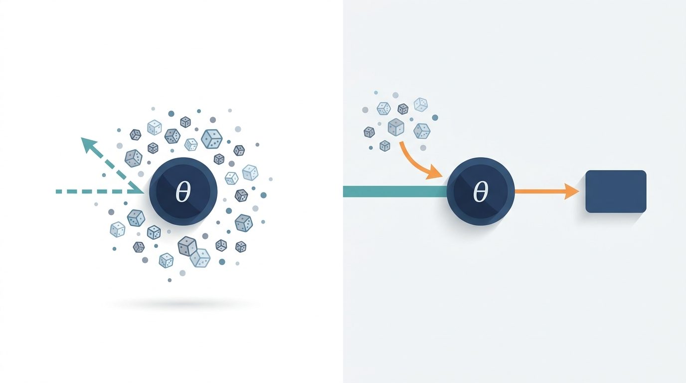
The reparameterization trick takes a fundamentally different approach. Instead of trying to push the gradient through a sampling operation, it redefines the sampling process itself so that randomness enters through a separate, independent channel.
The key insight is this: if a random variable can be expressed as a deterministic, differentiable function of some fixed noise source and the learnable parameters, then the gradient can flow through the deterministic transformation as naturally as it would through any other layer in a neural network.
Consider the Gaussian distribution as a concrete example. Rather than sampling directly from **N(μ, σ²)**, we sample a fixed noise variable **ε ~ N(0, 1)** and compute **z = μ + σ · ε**. Now θ appears only in the deterministic transformation μ(θ) and σ(θ), not in the noise source. The sampling step becomes just another operation in the computation graph, and standard automatic differentiation handles the rest.
With this reformulation, the gradient of the expectation simplifies to the expectation of the gradient—the derivative passes through the function f evaluated along the deterministic path z = g(θ, ε), using the ordinary chain rule. For each sampled noise value, we get a clean, low-noise estimate of how f changes as θ changes.
—
## A Concrete Numerical Illustration
To see the difference between these two estimators in action, consider a simple toy problem: estimating the gradient of **L(θ) = E[z²]** where **z ~ N(θ, 1)**. The true gradient is **2θ**, so for θ = 1.5, the correct answer is 3.0.
When we estimate this gradient using the score function approach with only 20 samples per estimate, the resulting distribution of gradient estimates has a mean of approximately 3.008 but a variance of 2.57. The estimates are unbiased but spread out—many individual estimates deviate substantially from the true value.
The reparameterization approach with the same 20 samples produces estimates with the same unbiased mean of 3.004, but with a variance of just 0.20. That’s roughly a **13-fold reduction** in variance for this straightforward example. The reparameterized estimates cluster tightly around the correct answer, giving the optimizer a clear, reliable direction to follow.
In the high-dimensional, often heavily-tailed posterior distributions that characterize real-world VAEs and variational inference problems, this gap widens considerably. It is this variance advantage that made scalable variational inference practical for the first time, enabling researchers to train deep generative models on complex datasets without resorting to more expensive sampling methods like Markov Chain Monte Carlo.
—
## When Reparameterization Is Possible—and When It Isn’t
The reparameterization trick is not universally applicable. It requires a differentiable path from the parameters to the sample, which not every probability distribution supports.
**Location-scale families**—including the Gaussian, logistic, Laplace, and uniform distributions—reparameterize naturally, as demonstrated above with the Gaussian example.
**Distributions with tractable inverse cumulative distribution functions** can be handled through inverse-transform sampling: draw a uniform random variable u and compute z as the inverse CDF evaluated at u, then differentiate through that inverse CDF with respect to the parameters.
**More complex continuous distributions** such as the Gamma, Beta, Dirichlet, and von Mises lack simple location-scale forms, but techniques like implicit reparameterization gradients can differentiate through their CDFs directly, avoiding the need for an explicit sampling path.
**Discrete random variables** present the most difficult case. A categorical or Bernoulli variable cannot be expressed as a continuous, differentiable function of its parameters—small changes in parameters don’t produce smooth changes in the sample. The standard workaround uses continuous relaxations: the Gumbel-Softmax (or Concrete) distribution replaces the hard discrete sample with a temperature-controlled continuous approximation that admits a reparameterized gradient, accepting a small bias in exchange for dramatically lower variance.
Even within fully reparameterizable models, additional variance reduction techniques exist. The “sticking the landing” method removes a residual score-function contribution that can leak into otherwise pathwise gradients as the approximate posterior converges toward the true posterior.
—
## Reparameterization in Real-World Applications
The reparameterization trick has become the engine behind several important families of models and algorithms:
**Variational Autoencoders** rely on reparameterization to obtain low-variance gradients of the ELBO with respect to the encoder network parameters. This is what made it possible to train deep VAEs using vanilla stochastic gradient descent, without custom optimization routines.
**Continuous-control reinforcement learning** algorithms, including Soft Actor-Critic, employ reparameterized policy gradients when the action space is continuous. By differentiating through the action selection process, these methods achieve far better sample efficiency than REINFORCE-style approaches, which must treat the action as an opaque black-box outcome.
**Bayesian deep learning and probabilistic programming** use reparameterized gradients to fit approximate posterior distributions over neural network weights via stochastic optimization, providing uncertainty estimates alongside predictions without the computational burden of MCMC sampling.
—
## Score Function vs. Pathwise Estimator: Head-to-Head Comparison
| Criterion | Score Function (REINFORCE) | Reparameterization (Pathwise) |
|—|—|—|
| Requires differentiable objective function | No | Yes |
| Requires differentiable sampling path | No | Yes |
| Handles discrete latent variables | Yes, natively | Only through continuous relaxations |
| Uses gradient information about the objective | No | Yes |
| Typical gradient variance | High | Low |
| Common application domains | Discrete action spaces, non-differentiable rewards | VAEs, continuous control, variational inference |
The reparameterization trick is not itself an optimization algorithm. Rather, it is a change of variables that converts the problem of “differentiating through a random sampling operation” into the much simpler problem of “differentiating through a deterministic function.” Whenever the underlying distribution permits such a transformation, the pathwise estimator should be strongly preferred for its far superior gradient signal.
—
## Frequently Asked Questions
**Q: Does the reparameterization trick always produce lower-variance gradients than REINFORCE?**
Not in every possible scenario. The variance advantage holds most strongly when the objective function f is smooth and locally well-approximated by its first-order Taylor expansion. If f is highly discontinuous or has sharp peaks that vary independently of the distribution parameters, the pathwise estimator may not benefit as much. However, for the vast majority of models used in deep learning—VAEs, Bayesian neural networks, continuous-control policies—f is smooth and the variance reduction is substantial.
**Q: Can I use both estimators together?**
Yes. In fact, some modern approaches combine the two. For example, when training a model with both discrete and continuous latent variables, one might use a relaxed (Gumbel-Softmax) reparameterization for the discrete variables and pathwise gradients for the continuous ones. Some estimators also blend score-function and pathwise components to capture complementary information, though care must be taken to avoid introducing bias.
**Q: Why does the score function estimator work at all if it’s so noisy?**
The score function estimator works because it is unbiased—its expected value equals the true gradient. Even though individual estimates are noisy, the law of large guarantees convergence given enough samples. In practice, variance reduction techniques like baseline subtraction (using a learned value function to center the reward) dramatically improve its usability, which is why policy-gradient methods in reinforcement learning remain active areas of research.
**Q: Is the reparameterization trick specific to Gaussian distributions?**
No. While the Gaussian case is the most widely used example, the principle applies to any distribution for which a differentiable sampling path can be constructed. The logistic, Laplace, and uniform distributions all reparameterize trivially. Many more complex distributions can be handled through inverse CDF methods or implicit differentiation techniques.
**Q: What happens to the reparameterization trick as the approximate posterior converges to the true posterior?**
As the approximate posterior becomes increasingly accurate, a subtle issue can arise: the score-function component of the gradient may not fully vanish, introducing variance back into what should be a purely pathwise gradient. The “sticking the landing” correction addresses this by removing this residual term, ensuring that the gradient estimator remains low-variance throughout training, not just at the beginning.
**Q: How does the reparameterization trick relate to the ELBO objective specifically?**
In a VAE, the ELBO contains an expectation over the approximate posterior distribution parameterized by the encoder. Computing the gradient of the ELBO with respect to the encoder parameters requires differentiating through this expectation. The reparameterization trick provides exactly the mechanism to do so—by making the sampling operation differentiable, it allows the reconstruction loss and the KL divergence regularization term to both contribute clean gradient signals to the encoder, enabling end-to-end training.
—
## Conclusion
The reparameterization trick stands as one of the most important methodological innovations in modern probabilistic machine learning. By recasting random sampling as a deterministic, differentiable transformation, it eliminates the fundamental obstacle that prevented gradient-based optimization through stochastic nodes. The resulting pathwise gradient estimator provides substantially lower variance than the score function alternative, translating directly into more stable training, faster convergence, and higher-quality generative models.
From variational autoencoders to Bayesian neural networks and continuous-control reinforcement learning agents, the reparameterization trick has proven to be an indispensable tool. Understanding why it works—and when it can be applied—is essential for anyone working with probabilistic generative models or stochastic optimization.
Thank you for reading
