



## Demystifying Fluid Flow: Simulating Kármán Vortices with the Lattice Boltzmann Method
The sight of alternating, swirling vortices trailing behind a blunt object in a flowing stream is one of the most iconic and recognizable patterns in all of physics. This intricate dance, known as a Kármán vortex street, is a staple of fluid dynamics, famously visible behind everything from bridge pillars and airplane wings to towering chimney stacks. For centuries, our understanding of such phenomena has been rooted in the Navier-Stokes equations—the fundamental laws governing fluid motion. However, what if I told you that you could generate this complex, beautiful pattern without explicitly solving a single one of those equations?
This article explores an alternative approach: the **Lattice Boltzmann Method (LBM)**. Instead of tackling the continuum-scale Navier-Stokes equations head-on, LBM takes a step back to the microscopic world. It treats a fluid not as a continuous substance, but as a statistical collection of particles colliding and streaming across a discrete lattice. The macroscopic phenomena we see—the pressure, the viscosity, and yes, even the Kármán vortex street—are not pre-programmed features but **emergent properties** that naturally arise from these simple, local interactions.
I developed the simulation presented here without solving a single partial differential equation. Instead, I implemented an LBM in C++ and ran it on the MareNostrum 5 supercomputer. The core insight is profound: LBM occupies a unique middle ground between molecular dynamics and traditional Navier-Stokes solvers, operating at a **mesoscopic** scale. It provides a powerful and elegant framework for simulating fluid flow, particularly in complex geometries and for low-Mach, subsonic conditions. The full source code for this project, including a simplified Python/NumPy version, is available on GitHub for anyone to explore.
### Why the Obvious Approach is Painful
The standard path to simulating a fluid begins with the **Navier-Stokes equations**. These are the conservation laws for mass, momentum, and energy, and they describe how a fluid’s velocity and pressure fields evolve over time. For simple, regular shapes like a flat plate in a channel, the math can be solved analytically. For the real world, with complex geometries like a car body, a porous rock, or a blood vessel, the equations become analytically intractable.
This is where computational fluid dynamics (CFD) comes in. Traditional CFD methods—like Finite Volume, Finite Difference, or Finite Element—discretize the domain into a computational mesh. They solve the Navier-Stokes equations at each point on this mesh. While powerful and mature, this approach carries a hidden, compounding cost: the mesh itself.
When you have a curved boundary—say, the cylinder in our simulation—creating an accurate computational grid becomes an engineering challenge in its own right. Body-fitted meshes must conform to the geometry, which is difficult to automate and can become prohibitively expensive. If the geometry changes, even slightly, the entire mesh often has to be regenerated. The physics problem is layered on top of a persistent mesh-generation problem.
LBM sidesteps this issue almost entirely. It doesn’t conform to the boundary; the boundary simply exists as a collection of grid points, and the physics are handled by intelligent rules at those points.
### A Different Starting Point: Statistical Mechanics
The fundamental shift in LBM lies in its question. Instead of asking, “What is the velocity field **u** at this point **x**?”, it asks, “How many particles are moving with velocity **cᵢ** at this point **x**?”
The central object in LBM is the **single-particle distribution function**, *f* (**x**, **v**, *t*). This function describes the expected number of particles at position **x** moving with velocity **v** at time *t*. The macroscopic properties we care about—density (ρ) and velocity (**u**)—are simply *moments* (averages) of this distribution.
The evolution of *f* is governed by the **Boltzmann equation**. It has two terms:
1. **Streaming**: Particles move ballistically, carrying their velocity distribution to a neighboring point.
2. **Collision**: Particles interact, redistributing their velocities and driving the system toward a state of equilibrium.
The challenge is the **collision operator**, Ω[*f*]. It’s a complex five-dimensional integral that encapsulates all possible particle interactions and scattering angles. For any real-world simulation, it is completely intractable.
### The One-Line Miracle: BGK
The breakthrough, known as the **BGK approximation** (after Bhatnagar, Gross, and Krook), is a stunningly simple solution. Instead of modeling the intricate details of every collision, the BGK model captures the *net effect*: collisions drive the distribution function *f* toward a local equilibrium state, *fᵉqᵇ*, at a rate determined by a single parameter, the **relaxation time (τ)**.
This is brilliant in its simplicity. The equilibrium distribution, *fᵉqᵇ*, is the familiar Maxwell-Boltzmann distribution from statistical mechanics. The collision term becomes a simple, scalar multiplication:
Ω[*f*] ≈ -(*f* – *fᵉqᵇ*) / τ
What does τ mean physically? It’s the average time it takes for the system to relax back to equilibrium after being disturbed. A large τ means a slow relaxation and a highly viscous fluid. A small τ means a fast relaxation and a “thinner” fluid. Through a mathematical procedure called the **Chapman-Enskog expansion**, it can be proven that the BGK equation recovers the Navier-Stokes equations exactly in the appropriate limit, with the kinematic viscosity (ν) related to τ by:
ν = *cₛ²* (τ – ½)
Here, *cₛ* is the lattice speed of sound. This is the key: **τ is the entire physical knob** for controlling viscosity in the simulation. You don’t set viscosity directly; you set τ. The NS equations are not assumed; they are **recovered** as the correct macroscopic limit of the kinetic Boltzmann description. This is the recurring theme of statistical mechanics: complex macroscopic behavior emerges from simple microscopic rules.
### From Continuous to Discrete: The D2Q9 Lattice
The Boltzmann equation still lives in a continuous velocity space. To build a computer simulation, we need a finite, discrete set of velocities. This is done using a **Taylor expansion** of *fᵉqᵇ* for flows where the bulk velocity **u** is small compared to the lattice speed of sound (the “low-Mach” assumption).
This leads to the **D2Q9** lattice, the workhorse of 2D LBM simulations. It consists of:
* **2 dimensions** (x, y)
* **9 discrete velocities**: one for “rest,” four for the cardinal directions (N, S, E, W), and four for the diagonals (NE, NW, SE, SW).
Each velocity direction *i* has a corresponding distribution function *fᵢ* and a fixed weight *wᵢ*, chosen to ensure the correct macroscopic properties (density and momentum) are recovered. For D2Q9, these weights are 4/9 for the center, 1/9 for the cardinal directions, and 1/36 for the diagonals. The lattice speed of sound is *cₛ* = 1/√3. The entire algorithm is built from these nine numbers.
### The Algorithm: Collision and Streaming
The LBM algorithm is breathtakingly simple, consisting of just two steps repeated in a loop:
1. **Collision**: At each lattice node, the distribution functions *fᵢ* are relaxed toward their equilibrium values *fᵉqᵢ* using the BGK operator. This is a purely local operation—no communication with neighbors is needed.
2. **Streaming**: Each distribution function *fᵢ* is moved (“streamed”) from its current node to its neighboring node in the direction of *cᵢ*.
This interplay between a local collision step and a non-local streaming step is what creates fluid dynamics. The collision step introduces viscosity and diffusion, while the streaming step transports information across the grid.
The implementation is highly parallel. Because collision is local and streaming only involves reading from immediate neighbors, the algorithm is **embarrassingly parallel**. It maps perfectly onto modern hardware, from multi-core CPUs to thousands of GPU cores.
### Boundary Conditions: Complex Geometry for Free
One of the greatest strengths of LBM is its treatment of boundaries. After the streaming step, some distribution functions at nodes next to a solid wall are “missing”—they would have arrived from inside the solid, which contains no fluid. These missing populations are handled by **boundary conditions**.
The most common and elegant condition is **bounce-back**. Any population streaming into a solid node is simply reflected back in the opposite direction. *fᵢ* at the wall becomes *fᵢ* at the adjacent fluid node.
This simple rule has a remarkable consequence: **any obstacle shape is just a boolean flag**. To place a cylinder in your flow, you simply mark the lattice nodes that fall inside the cylinder as “solid.” The bounce-back rule automatically applies the correct no-slip boundary conditions at every point of the interface, with no mesh generation, no stencil corrections, and no changes to the core algorithm. The wall sits halfway between the last fluid node and the solid node, providing second-order accuracy.
### Results: From Steady Flow to Kármán Vortices
Our simulation domain is a 400×400 lattice with a circular cylinder obstacle. The inlet velocity (*uₓ*) is set to 0.1 in lattice units, ensuring we remain in the low-Mach regime. The behavior of the flow is dramatically different depending on the relaxation time τ.
**At τ = 0.75 (low Reynolds Number, Re ≈ 96):**
The wake behind the cylinder is steady and symmetric. The collision frequency is high, so the distribution function is quickly damped toward equilibrium. The flow is highly viscous and laminar, with no persistent structure in the wake.
**At τ = 0.55 (Higher Reynolds Number, Re ≈ 480):**
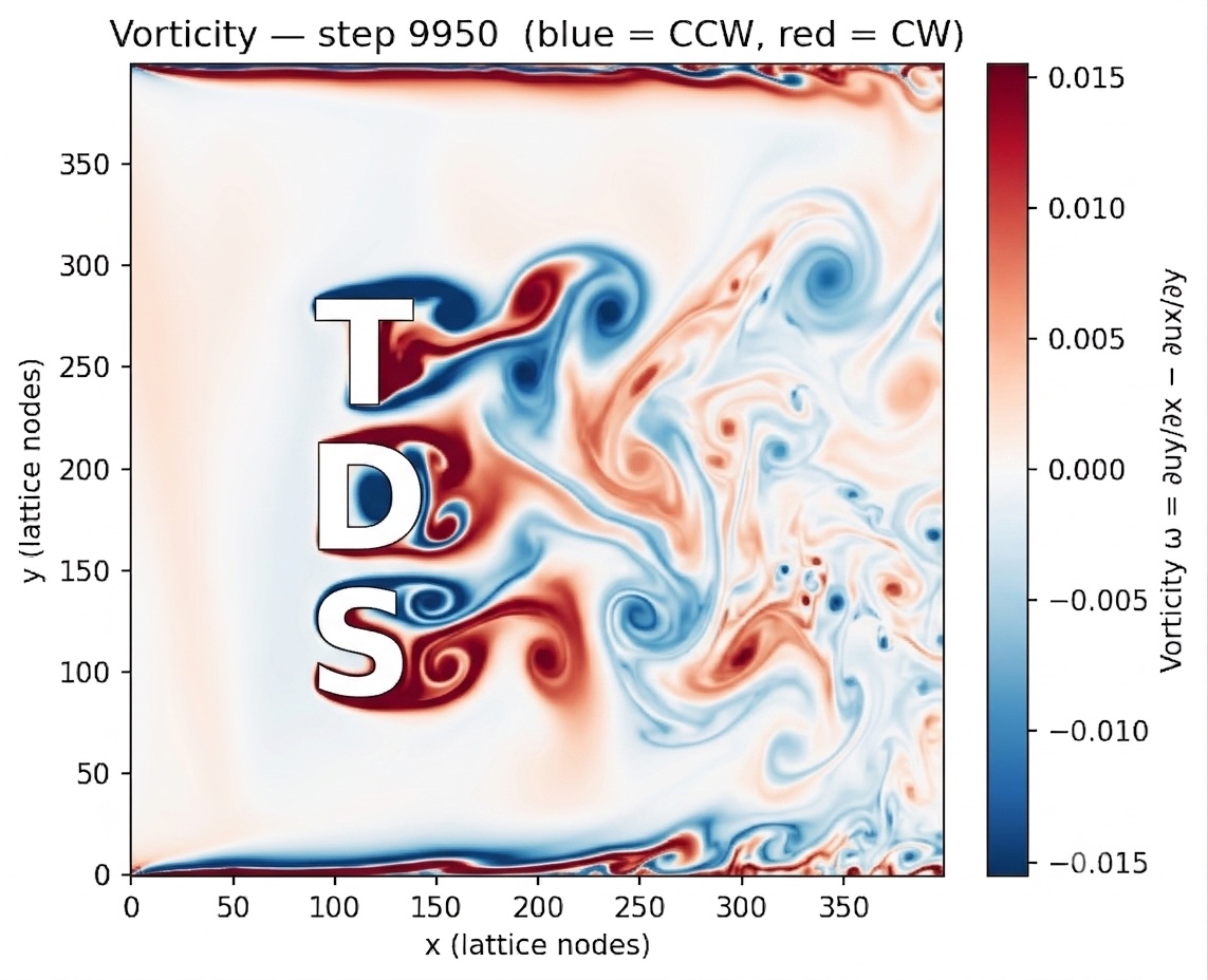
The physics changes completely. Here, the simulation beautifully reproduces the **Kármán vortex street**. Vortices shed alternately from the top and bottom surfaces of the cylinder.
This is the crucial insight. From a statistical mechanics perspective, this vortex shedding is driven by the **departure of *f* from its equilibrium shape**. At the lower τ, collisions are too fast to dampen perturbations. The non-equilibrium part of the distribution function, *f* – *fᵉqᵇ*, grows large enough to feed back into the macroscopic momentum field, creating a sustained oscillation. A perfectly equilibrium fluid would be unable to produce this structure.
The Boolean-flag approach to boundaries means that changing the geometry requires no algorithmic changes. The same code, with only the solid-node map changed, can simulate a wide variety of complex flows. The resulting visualizations show intricate vortex interactions and multi-body flow phenomena.
### Scaling to MareNostrum 5
The algorithm’s design makes it ideal for massive parallelization. With OpenMP pragmas on the collision and streaming loops, we scaled the solver across a full node of the **MareNostrum 5** supercomputer at the Barcelona Supercomputing Center.
The results show three distinct performance regimes:
* **1 to 32 threads:** Excellent strong scaling, with efficiency above 75% and a 24.6x speedup.
* **64 threads:** Efficiency drops to 42% as the memory bus becomes saturated.
* **112 threads (full node):** Performance actually *falls*, as memory access latency across two CPU sockets negates the benefits of additional cores.
A critical optimization was switching from a “push” to a “**pull**” streaming scheme. This eliminates **false sharing**, a major performance bottleneck where multiple threads compete to update adjacent memory locations. The pull scheme is significantly faster and more scalable.
A key takeaway is the impact of the code itself. A well-optimized, single-threaded LBM with pull streaming runs in **31.7 seconds**, a **3.6x speedup** over an unoptimized push implementation that took 113 seconds. This gain came from improving the memory access pattern alone, before any parallelism was even considered.
### When to Use LBM (and When Not To)
LBM is an excellent choice when:
* The geometry is complex or evolves over time.
* You need to leverage massively parallel hardware (CPUs, GPUs).
* You are interested in mesoscale phenomena, such as slip at walls.
* You are building a foundation for multiphase or multicomponent flows.
It is less suitable for:
* High-Mach flows (above ~Mach 0.3), where the low-order Taylor expansion for *fᵉqᵇ* breaks down.
* Very high Reynolds number flows, as the stability constraint (τ > 0.5) limits how low the viscosity can be set.
* Problems where absolute physical unit calibration is critical from the very beginning.
### What’s Next: Multiphase Flows with Shan-Chen
This simulation addressed a single-component, single-phase fluid. Many of the most interesting problems involve two or more immiscible fluids, such as oil and water, rising bubbles, or droplet formation.
The **Shan-Chen model** is the natural next step. It extends LBM to handle multiphase flows by introducing short-range inter-particle forces. These forces create an effective equation of state, causing phase separation and generating interfacial tension directly from the collision dynamics, rather than being imposed externally.
In the next article, I will derive the Shan-Chen model, extend our current solver, and visualize what happens when you let two fluids compete for the same lattice space.
### Closing Thought
What I find most satisfying about LBM is how it makes the relationship between scales tangible. The Navier-Stokes equations feel fundamental because they describe the world we see. But LBM reveals them for what they are: a statistical consequence of countless microscopic collisions.
Viscosity isn’t a parameter you input; it’s a collision timescale. The Kármán vortex street isn’t a numerical instability you code for; it’s what emerges when the fluid’s inertia overcomes its viscosity. Every macroscopic pattern in the simulation has a direct, microscopic interpretation in the underlying statistical mechanics.
LBM builds a concrete bridge between these scales, made tangible in a few hundred lines of C++. That is its true power.
### References
For those interested in diving deeper, here are the key resources:
* **Mohamad, A.A. (2019).** *Lattice Boltzmann Method: Fundamentals and Engineering Applications with Computer Codes*. Springer.
* **Krüger, T. et al. (2017).** *The Lattice Boltzmann Method: Principles and Practice*. Springer.
* **Bhatnagar, P.L., Gross, E.P., & Krook, M. (1954).** A Model for Collision Processes in Gases. *Physical Review*, 94(3), 511–525.
* **Chapman, S., & Cowling, T.G. (1970).** *The Mathematical Theory of Non-Uniform Gases*. Cambridge University Press.
