



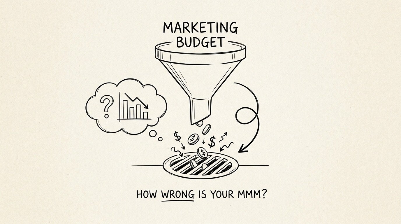
# Why Your Marketing Mix Model Can’t Tell Channels Apart — And How to Fix It
## The Measurement Problem Nobody Talks About Enough
Marketing leaders spend enormous budgets across dozens of channels and then rely on statistical models to answer a deceptively simple question: how much did each channel actually contribute? Marketing Mix Modelling (MMM) has become the go-to framework for answering this, powered by open-source tools from major technology companies that make running a model easier than ever before. But running a model and trusting it are two entirely different things.
The core difficulty isn’t a missing algorithm or a more sophisticated prior distribution. It is a data problem. Marketing budgets are planned in unison, rise and fall with business demand, and rarely venture far from their historical ranges. That narrow band of spend patterns means the model is trying to disentangle channels that never truly moved independently. The result is estimates that could swing wildly depending on the version of reality you happen to be looking at.
## Three Distinct Failures, One Root Cause
When an MMM produces unreliable results, the failure typically falls into one of three categories. Each one stems from a different kind of missing variation in the underlying spend data.
### 1. Channel Variance: The Model Can’t Separate What Never Moved Apart
Marketing channels are almost always allocated in the same planning cycle. They rise together during growth periods and contract together during tightening months. Because no channel ever moves on its own, the regression simply cannot distinguish their individual effects. The estimates carry enormous variance — refit the model on a slightly different version of the same data, and the answer could land anywhere. Any channel could emerge as the top performer, regardless of its true contribution.
### 2. Selection Bias: Spend Follows Demand, and the Model Pays the Price
Organisations naturally allocate more marketing budget when demand is strong. Since demand itself is never directly observed, the model relies on proxies like category search volume. When those proxies fall short, the residual gets absorbed by the channel coefficients. This is textbook omitted variable bias, and unlike variance, it does not disappear with more data. More observations of a mis-specified relationship just produce a more confident estimate of the wrong number.
### 3. Curve Shape Identification: Adstock and Saturation Blur Together
Every MMM must simultaneously estimate how quickly a channel’s returns diminish (saturation) and how long its effects persist (adstock). A recent study found that these shape parameters are frequently not separately identifiable from ordinary weekly spend data. To tell a bending curve from a straight line, a channel needs to be observed at clearly different spend levels while other channels hold steady. When everything moves in lockstep, a curve and a line fit the data equally well.
## Why More Data Doesn’t Solve This
A common response to any of these three problems is to collect more data — longer time horizons, additional observations, more granular tracking. But here is the uncomfortable truth: more weeks of correlated spend simply give you a tighter estimate of the same confused answer. The model sees the same pattern repeated and becomes more precise about a result that was wrong to begin with.
The industry has also increasingly turned to incrementality testing and geo-experiments to calibrate models. These are valuable tools, but they tend to read one channel at a time, require months of planning and execution, and recent research suggests that many open-source geo-testing tools report a false positive lift 14 to 30 percent of the time.
## The Fix: Spend That Carries More Information
Step back and all three failures share the same remedy. The model needs spend that varies in the specific ways it requires to answer each question. Variance needs channels moving independently. Bias needs spend changes that have nothing to do with demand. Saturation needs periods of high spend held long enough to register. Adstock needs changes sustained beyond the carryover window.
This can be achieved without increasing the total budget. A budget phasing algorithm rearranges when money is spent, not how much is spent. Think of it as redesigning the timing schedule so that the data the model learns from contains the variation it actually needs.
## How a Phasing Algorithm Works
The concept starts with a simple principle: each channel should, at various points during the planning period, spend money for reasons unrelated to overall demand. This is achieved through several coordinated tactics.
**Independent movement.** Channels are nudged up and down on different weeks so that they do not all peak and trough at the same time. Random variation drawn separately for each channel achieves this.
**Dark periods.** A channel can be taken offline entirely for a sustained stretch — typically four weeks — with its budget redistributed to other periods. This creates a natural experiment within the data and helps identify both adstock carryover and selection bias.
**Surge periods.** A channel can be pushed well above its normal level for an entire month, absorbing budget freed up during dark periods or drawn from smaller cuts in other weeks. This gives the model the high-spend observations it needs to pin down saturation curves.
Crucially, all of this happens within the same annual budget. No additional spend is required. The only change is the timing.
## What the Evidence Shows
Simulation studies testing these approaches on realistic scenarios have produced striking results. When channels are phased according to a combined strategy that applies all three tactics, the model’s performance improves dramatically across every diagnostic:
The range of possible estimates for each channel’s contribution tightens substantially. The point estimates shift toward their true values rather than being systematically inflated by demand-following behavior. And the saturation and adstock curves become identifiable in ways they were not with unphased data.
The trade-off is real but measured. Rearranging spend across the calendar means some money gets shifted to periods where returns are lower, simply because the response curve flattens at higher spend levels. The cost of this rearrangement has been quantified at roughly three to four percent of the revenue driven by the phased channels — a price that, in most cases, is dwarfed by the value of knowing what those channels actually contribute.
## Does This Approach Scale?
One of the practical concerns with any scheduling intervention is whether it remains effective as the number of channels grows. With four channels, there is enough flexibility to stagger dark periods and surges without overlap. With fifteen channels, the scheduling becomes more constrained, and the gains do shrink somewhat — but they remain meaningful. The same budget phasing approach continues to deliver measurable improvements in variance reduction, bias correction, and curve identifiability even as the complexity of the channel mix increases.
## What This Means for Your Team
If you are running a marketing mix model today, the most important question is not whether your model is technically sophisticated. It is whether your spend data contained the information needed to answer the questions you are asking of it. A Bayesian model with flexible priors cannot invent variation that was never present. A hierarchical model with regional breakdowns cannot help if the channels in every region still move in lockstep.
The path forward is not more modeling — it is more informative data. Budget phasing is a practical, budget-neutral method for generating that information. It changes only the timing of existing spend to give the model the independent movement, the demand-independent variation, and the spend-level diversity it needs to produce reliable answers.
—
## Frequently Asked Questions
**What exactly does a phasing algorithm change?**
It changes the weekly distribution of each channel’s spend throughout the year. The annual total stays exactly the same. What changes is which weeks see higher spend and which weeks see lower spend, and whether channels move independently of one another.
**Do I need to change how I work with my media agency?**
You need to hand them a weekly spend plan instead of a monthly or annual one. The channels and their annual budgets remain the same. The difference is that some weeks will look busier and others quieter than a conventional even distribution would suggest. The agency still buys the same total volume.
**What if my channel is booked far in advance and cannot be phased?**
Television and other upfront-buy media are the most common example. In practice, you can apply lighter phasing to those channels and reserve the more aggressive dark periods and surges for channels with more flexible scheduling, such as digital paid social and search. Even partial phasing across some channels improves the data quality for the entire model.
**How long does it take to see the benefits?**
The gains accumulate as more of the historical data window is phased. If you begin phasing next year, the model trained on next year’s phased data plus the two prior years will already benefit. The full payoff arrives once the entire training window contains phased spend, typically after two to three years of consistent phasing.
**Is this the same as a holdout or geo-experiment?**
No. A geo-experiment withholds spend from an entire region and compares it to a treated region. Phasing is an internal data restructuring technique that works within your existing spend pattern. The two approaches complement each other — phasing improves the data for your ongoing model, while geo-experiments provide direct causal validation for specific channels.
**Can I use this with any MMM tool?**
Yes. The approach works with any model that takes weekly spend as input and estimates channel contributions. It is tool-agnostic because it changes the input data, not the model itself. Open-source packages are now available that can simulate what improved estimates would look like given your specific channel mix and response assumptions.
**What happens if demand itself changes during the year in unpredictable ways?**
The phasing schedule is drawn in advance and is demand-independent by design. If an unexpected demand shock occurs, the actual spend may deviate from the planned schedule. The model benefits from the planned variation, and real-world deviations add additional noise but do not undo the structural improvement the phasing provides.
**Is three years of data enough?**
Three years of weekly data is a standard choice for MMM because it balances having enough observations with keeping the data relevant. Phasing does not change this requirement. However, the value of each year of phased data is higher than the value of each year of unphased data, because the information content per observation is greater.
—
## Conclusion
Marketing Mix Modelling remains one of the most valuable tools for understanding how marketing investments translate into business outcomes. But its reliability depends entirely on the quality and structure of the input data. When channels are planned together, follow demand, and stay within familiar ranges, no amount of modeling sophistication can fully compensate for the missing variation.
Budget phasing addresses the problem at its source. By rearranging the timing of existing spend, it introduces the independent movement, the demand-independent changes, and the varied spend levels that models need to separate channels, correct bias, and identify response curves. The cost is modest and measurable — typically a few percent of channel-attributed revenue — and the payoff is a model you can actually trust.
The lesson from the evidence is clear: it was never the model’s fault. The data just never gave it a fair chance. Budget phasing is how you change that.
Thank you for reading
