



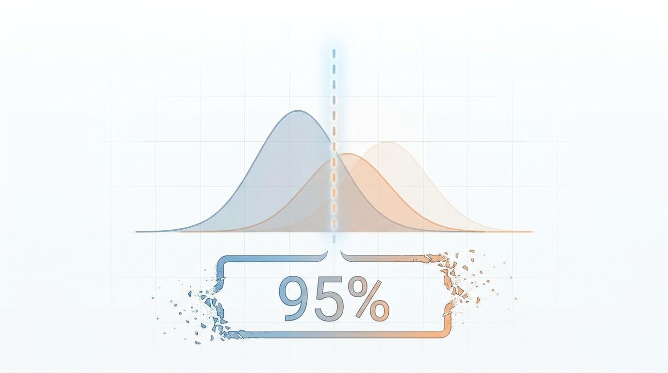
# What the “95%” in Your Results Actually Means — And Why Everyone Gets It Wrong
## The Question That Stumps Almost Every Stakeholder
Imagine this scenario. You’ve just finished reviewing an experiment comparing two versions of a checkout flow. The new version shows a lift of 0.3 percentage points in conversion, and the analysis confirms that the result is statistically significant at the 95% level. A product manager leans over and asks:
“So does this mean there’s a 95% chance the new flow is actually better?”
The room goes quiet. People nod, but nobody wants to be the one to answer.
Here’s why that silence matters: the answer is no — not in the way most people hear it. And that single misunderstanding has quietly distorted decisions across healthcare, technology, and financial services for decades. The number 95% is attached to something very different from what intuition suggests, and once you understand what it actually refers to, you’ll never look at an experiment result the same way again.
—
## The Origin Story Behind the Confidence Interval
The statistical framework behind what we now call a “confidence interval” was formalized by Jerzy Neyman between 1934 and 1937. Neyman was grappling with a fundamental challenge: any claim we make about an unknown quantity has to be built from data that could have turned out differently. Run the same study with a new batch of participants, and you get a different estimate, a different range, a different conclusion.
His solution was to shift the question entirely. Instead of asking, “Where does the true value sit?”, he asked, “How often does my method hit the target?” A 95% confidence interval is constructed so that, if you repeated the entire data-collection process many times, 95% of the intervals you produced would capture the true underlying value. That’s a claim about the reliability of the method over the long run — not a statement about any individual interval you compute from a single dataset.
The mathematics for estimating a population mean follows naturally from the Central Limit Theorem. When you have a large enough sample, the sample mean approximates a normal distribution around the true population mean. By rearranging the probability statement to isolate the unknown parameter, you arrive at the familiar formula that bounds the range above and below your observed estimate. The randomness in this expression lives entirely in the sample mean — not in the parameter itself. Once you substitute your actual observed numbers, the interval becomes fixed. It either includes the true value or it doesn’t. The 95% describes how the procedure behaves across hypothetical repetitions, not what you can assert about this particular output.
This distinction is so counterintuitive that surveys of professional scientists have repeatedly found that large majorities interpret confidence intervals as probability statements about the parameter being inside a specific interval. That interpretation is precisely what Neyman’s framework was designed to rule out.
—
## The Alternative: What Bayesian Intervals Actually Tell You
There’s another school of thought that asks a fundamentally different question. Rather than interrogating the long-run behavior of a procedure, the Bayesian approach asks: “Given what I’ve observed and what I already believed beforehand, what should I now believe?”
To answer this, you start with a prior distribution that encodes your existing knowledge or assumptions about the parameter. When new data arrive, Bayes’ theorem combines this prior with the likelihood of observing what you saw, producing an updated posterior distribution. A credible interval is simply the narrowest range that accumulates 95% of the posterior probability mass.
Because this is a direct probability statement about the parameter itself, it feels much more natural. You can honestly say, “Given the data and my prior, there’s a 95% probability the true effect falls in this range.” The tradeoff is that the answer depends on what prior you chose. Two analysts examining identical data but holding different prior beliefs will arrive at different credible intervals — and both are technically correct within their own frameworks.
Frequentist methods were developed in part to sidestep this subjectivity. A confidence interval’s coverage guarantee holds regardless of anyone’s preexisting beliefs, because the framework deliberately excludes priors from the calculation. Whether that’s a feature or a limitation depends entirely on the decision you’re trying to make.
—
## Seeing the Difference in Practice: A Churn Analysis
Consider a subscription product with a monthly churn rate of 1.50%. After deploying a change to the billing experience, you observe 350 churned users out of 20,000 active accounts in a given month. That’s an observed rate of 1.75% — a gap of 0.25 percentage points from the predicted baseline.
A frequentist analysis proceeds by asking what the standard error of this observed rate would be if the underlying model were correctly calibrated. The test statistic comes out to roughly 2.9, which translates into a two-sided p-value below 0.01. The resulting confidence interval for the gap is approximately 0.08 to 0.42 percentage points, entirely above zero. By the standards of this procedure, the model’s predictions are miscalibrated and the new billing experience has a detectable effect.
Now switch to a Bayesian lens. With a weak prior — say, a normal distribution centered at zero with a standard deviation of 1 percentage point — the data overwhelm the prior, and the posterior credible interval nearly mirrors the frequentist result: roughly 0.08 to 0.42 percentage points. The conclusion is the same.
But change the prior. Suppose five years of monitoring has shown this product segment to be remarkably stable, and you encode that strong belief with a prior centered at zero with a standard deviation of just 0.05 percentage points. Now the posterior mean gets pulled sharply toward zero, and the credible interval becomes approximately negative 0.02 to positive 0.15 percentage points. Zero is inside that range. The same data, the same sample size, and the same observed counts — but a completely different conclusion.
This isn’t a bug. It’s the logical consequence of choosing which question you want your statistical output to answer.
—
## Why Bigger Samples Don’t Always Mean Better Answers
One of the most disorienting phenomena in applied statistics is what happens when you let sample sizes grow very large. As the number of observations increases, the standard error of any estimate shrinks proportionally to the square root of the sample size. That means even tiny, practically meaningless differences become statistically “significant” — they cross the threshold that a hypothesis test uses to reject the null.
This creates a dangerous disconnect for product teams running experiments on high-traffic platforms. An A/B test on a feature used by millions of users might declare a statistically significant lift of 0.02 percentage points — a gap so small it would be invisible in any business metric dashboard and utterly irrelevant to the product roadmap. Yet the procedure will confidently report it as real.
The frequentist framework is not wrong here. It is answering the question it was designed to answer: “Is there any detectable deviation from the null?” But the analyst’s actual question is almost always more nuanced: “Is this deviation large enough to justify changing anything?” Treating a statistical finding as an automatic business recommendation, without evaluating whether the magnitude of the effect is material, is where real damage happens.
—
## Choosing the Right Framework for the Decision at Hand
Neither approach is universally superior. They serve different purposes and answer different questions.
Confidence intervals shine when you need objectivity and reproducibility. Regulatory environments, randomized controlled trials in medicine, and the default pipelines of A/B testing platforms all lean on frequentist methods because the guarantee — “this procedure will be right 95% of the time in the long run” — doesn’t depend on anyone’s opinion. Any analyst running the same code on the same data should reach the same conclusion, and that consistency is valuable.
Bayesian reasoning becomes essential when accumulated domain knowledge matters. An experienced analyst who has seen dozens of metric fluctuations come and go carries information that no single dataset can capture. That prior knowledge — “gaps like this have historically resolved themselves within two weeks” — is a legitimate form of evidence, and the Bayesian framework is the formal way to integrate it with new observations.
The practical path forward is not to pick one and discard the other. It’s to use each for the question it genuinely answers: frequentist tests as an objective checkpoint that any reviewer would independently verify, and Bayesian thinking as the lens through which you decide how much that checkpoint result should reshape your actual beliefs and actions.
—
## Practical Guidelines for Everyday Use
– **Define materiality before you look at results.** Know in advance what size of effect would genuinely influence a product decision. A result can be statistically significant without being strategically relevant.
– **Never treat a p-value or confidence interval as a verdict on its own.** Statistical significance on large samples is a trigger for deeper investigation, not a green light for action.
– **Take disagreements between your prior expectations and the data seriously.** A stark mismatch could signal a genuine shift in user behavior, a data quality problem, or an overly narrow prior — all of which warrant attention.
– **Label your intervals accurately.** A confidence interval and a credible interval are not synonyms, and reporting one as the other is making a claim that your method cannot actually support.
– **When in doubt, describe the uncertainty in plain language.** Explain what the interval means, what question it answers, and what assumptions went into it. Stakeholders who understand the limitations make better decisions than those who only see a number.
—
## Frequently Asked Questions
**Q: If I can’t say “there’s a 95% chance the true value is in this interval,” what CAN I say?**
A: You can say, “The procedure I used to build this interval will capture the true value 95% of the time if I were to repeat the entire experiment many times.” That’s a statement about the method’s track record, not about this particular output.
**Q: Is a Bayesian approach always better because it gives a more intuitive answer?**
A: Not necessarily. The Bayesian answer depends on your prior, which means different people can reach different conclusions from the same data. In regulated settings or when objectivity and reproducibility are paramount, the frequentist approach’s independence from prior beliefs is a serious advantage.
**Q: How do I choose the right prior for a Bayesian analysis?**
A: A good prior reflects genuinely held knowledge or reasonable assumptions about the parameter before seeing the new data. When there is little prior information, a weakly informative prior (with a large spread) lets the data dominate the result. The key is to document and justify the prior choice transparently.
**Q: Does the Jeffreys-Lindley paradox mean frequentist tests are broken?**
A: No. It highlights a genuine tension that arises when sample sizes are very large. The frequentist test is doing exactly what it was designed to do — detecting deviations, no matter how small. The issue is that detecting a deviation and finding it meaningful are two separate questions, and conflating them leads to poor decisions.
**Q: Should I always report both a frequentist and Bayesian result?**
A: It depends on your audience and context. For internal product reviews, showing both can be illuminating because it highlights where prior assumptions matter and where the data speak for themselves. For regulated or published work, follow the conventions of your field and clearly state which framework you’re using.
—
## Conclusion
The gap between what statistical outputs actually mean and what most people believe they mean is one of the most persistent and consequential misunderstandings in data-driven decision-making. A confidence level is a property of the method, not a probability statement about your specific result. A credible interval gives you the direct probability interpretation you might expect — but only once you’ve made your prior commitments explicit. And neither framework, on its own, tells you whether a statistically detectable difference matters in practice.
The analysts and teams that navigate this landscape effectively are the ones who treat statistical tools as what they are: precise instruments that answer precise questions, surrounded by judgment and context that no formula can replace. Understanding the machinery doesn’t make you a slave to it. It makes you the kind of analyst who can explain what the numbers really say — and, just as importantly, what they don’t.
Thank you for reading
