Constructing Sensible MLOps for a Private ML Undertaking

# Introduction

 
You’ve most likely completed your fair proportion of information science and machine studying initiatives.

They’re nice for sharpening abilities and displaying off what and have realized. However right here’s the factor: they usually cease wanting what real-world, production-level information science appears like.

On this article, we take a mission — the U.S. Occupational Wage Evaluation — and switch it into one thing that claims, “This is ready for real-world use.”

For this, we’ll stroll via a easy however stable machine studying operations (MLOps) setup that covers the whole lot from model management to deployment.

It’s nice for early-career information individuals, freelancers, portfolio builders, or whoever desires their work to appear to be it got here out of an expert setup, even when it didn’t.

On this article, we’ll transcend pocket book initiatives: we’ll arrange our MLOps construction, learn to arrange reproducible pipelines, mannequin artifacts, a easy native software programming interface (API), logging, and eventually, produce helpful documentation.

Picture by Creator

# Understanding the Job and the Dataset

 
The state of affairs for the mission consists of a nationwide U.S. dataset that has annual occupational wage and employment information in all 50 U.S. states and territories. The info particulars employment totals, imply wages, occupational teams, wage percentiles, and in addition geographic identifiers.

Your principal goals are:

• Evaluating variations in wages throughout totally different states and job classes
• Working statistical checks (T-tests, Z-tests, F-tests)
• Constructing regressions to know the connection between employment and wages
• Visualizing wage distributions and occupation developments

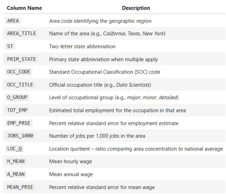
Some key columns of the dataset:

• OCC_TITLE — Occupation title
• TOT_EMP — Complete employment
• A_MEAN — Common annual wage
• PRIM_STATE — State abbreviation
• O_GROUP — Occupation class (Main, Complete, Detailed)

Your mission right here is to supply dependable insights about wage disparities, job distribution, and statistical relationships, but it surely doesn’t cease there.

The problem can be to construction the mission in a means that it turns into reusable, reproducible, and clear. This can be a crucial ability required for all information scientists these days.

# Beginning with Model Management

 
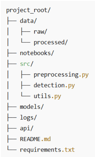
Let’s not skip the fundamentals. Even small initiatives deserve a clear construction and correct model management. Right here’s a folder setup that’s each intuitive and reviewer-friendly:

A number of finest practices:

• Maintain uncooked information immutable. You do not want to the touch it, simply copy it for processing.
• Think about using Git LFS in case your datasets get huge and chunky.
• Maintain every script in src/ centered on one factor. Your future self will thanks.
• Commit usually and use clear messages like:
  feat: add T-test comparability between administration and manufacturing wages.

Even with this straightforward construction, you might be displaying hiring managers that you simply’re considering and planning like an expert, not like a junior.

# Constructing Reproducible Pipelines (and Leaving Pocket book Chaos Behind)

 
Notebooks are superb for exploration. You strive one thing, tweak a filter, re-run a cell, copy a chart, and earlier than it, you’ve obtained 40 cells and no concept what really produced the ultimate reply.

To make this mission really feel “production-ish”, we’ll take the logic that already lives within the pocket book and wrap it in a single preprocessing perform. That perform turns into the one, canonical place the place the U.S. occupational wage information is:

• Loaded from the Excel file
• Cleaned and transformed to numeric
• Normalized (states, occupation teams, occupation codes)
• Enriched with helper columns like whole payroll

From then on, each evaluation — plots, T-tests, regressions, correlations, Z-tests — will reuse the identical cleaned DataFrame.

// From Prime-of-Pocket book Cells to a Reusable Operate

Proper now, the pocket book roughly does this:

• Hundreds the file: state_M2024_dl.xlsx
• Parses the primary sheet right into a DataFrame
• Converts columns like A_MEAN, TOT_EMP to numeric
• Makes use of these columns in:
  • State-level wage comparisons
  • Linear regression (TOT_EMP → A_MEAN)
  • Pearson correlation (Q6)
  • Z-test for tech vs non-tech (Q7)
  • Levene check for wage variance

We’ll flip that right into a single perform referred to as preprocess_wage_data which you could name from wherever within the mission:

from src.preprocessing import preprocess_wage_data
df = preprocess_wage_data("data/raw/state_M2024_dl.xlsx")

Now your pocket book, scripts, or future API name all agree on what “clean data” means.

// What the Preprocessing Pipeline Truly Does

For this dataset, the preprocessing pipeline will:

1. Load the Excel file as soon as.

xls = pd.ExcelFile(file_path)
df_raw = xls.parse(xls.sheet_names[0])
df_raw.head()

2. Convert key numeric columns to numeric.

These are the columns your evaluation really makes use of:

• Employment and depth: TOT_EMP, EMP_PRSE, JOBS_1000, LOC_QUOTIENT
• Wage measures: H_MEAN, A_MEAN, MEAN_PRSE
• Wage percentiles: H_PCT10, H_PCT25, H_MEDIAN, H_PCT75, H_PCT90, A_PCT10, A_PCT25, A_MEDIAN, A_PCT75, A_PCT90

We coerce them safely:

df = df_raw.copy()
numeric_cols = [
        "TOT_EMP", "EMP_PRSE", "JOBS_1000", "LOC_QUOTIENT" ….]
for col in numeric_cols:
        if col in df.columns:
            df[col] = pd.to_numeric(df[col], errors="coerce")

If a future file accommodates bizarre values (e.g. ‘**’ or ‘N/A’), your code won’t explode, it’s going to simply deal with them as lacking, and the pipeline won’t break.

3. Normalize textual content identifiers.

For constant grouping and filtering:

• PRIM_STATE to uppercase (e.g. “ca” → “CA”)
• O_GROUP to lowercase (e.g. “Major” → “major”)
• OCC_CODE to string (for .str.startswith("15") within the tech vs non-tech Z-test)

4. Add helper columns utilized in analyses.

These are easy however helpful. The helper for the full payroll per row is, approximate, utilizing the imply wage:

 df["TOTAL_PAYROLL"] = df["A_MEAN"] * df["TOT_EMP"]

The wage-to-employment ratio is helpful for recognizing excessive wage / low employment niches, with safety towards division by zero:

 df["WAGE_EMP_RATIO"] = df["A_MEAN"] / df["TOT_EMP"].substitute({0: np.nan})

5. Return a clear DataFrame for the remainder of the mission.

Your later code for:

1. Plotting high/backside states
2. T-tests (Administration vs Manufacturing)
3. Regression (TOT_EMP → A_MEAN)
4. Correlations (Q6)
5. Z-tests (Q7)
6. Levene’s check

can all begin with:

 df = preprocess_wage_data("state_M2024_dl.xlsx")

Full preprocessing perform:

Drop this into src/preprocessing.py:

import pandas as pd
import numpy as np
def preprocess_wage_data(file_path: str = "state_M2024_dl.xlsx") -> pd.DataFrame:
    """Load and clear the U.S. occupational wage information from Excel.
    - Reads the primary sheet of the Excel file.
    - Ensures key numeric columns are numeric.
    - Normalizes textual content identifiers (state, occupation group, occupation code).
    - Provides helper columns utilized in later evaluation.
    """
    # Load uncooked Excel file
    xls = pd.ExcelFile(file_path)

Test the remainder of the code right here.

# Saving Your Statistical Fashions and Artifacts

 
What are mannequin artifacts? Some examples: regression fashions, correlation matrices, cleaned datasets, and figures.

import joblib
joblib.dump(mannequin, "models/employment_wage_regression.pkl")

Why save artifacts?

• You keep away from recomputing outcomes throughout API calls or dashboards
• You protect variations for future comparisons
• You retain evaluation and inference separate

These small habits elevate your mission from exploratory to production-friendly.

# Making It Work Regionally (With an API or Tiny Net UI)

 
You don’t want to leap straight into Docker and Kubernetes to “deploy” this. For lots of real-world analytics work, your first API is just:

• A clear preprocessing perform
• A number of well-named evaluation features
• A small script or pocket book cell that wires them collectively

That alone makes your mission straightforward to name from:

• One other pocket book
• A Streamlit/Gradio dashboard
• A future FastAPI or Flask app

// Turning Your Analyses Right into a Tiny “Analysis API”

You have already got the core logic within the pocket book:

• T-test: Administration vs Manufacturing wages
• Regression: TOT_EMP → A_MEAN
• Pearson correlation (Q6)
• Z-test tech vs non-tech (Q7)
• Levene’s check for wage variance

We’ll wrap a minimum of one among them right into a perform so it behaves like a tiny API endpoint.

Instance: “Compare management vs production wages”

This can be a perform model of the T-test code that’s already within the pocket book:

from scipy.stats import ttest_ind
import pandas as pd
def compare_management_vs_production(df: pd.DataFrame):
    """Two-sample T-test between Management and Production occupations."""
    # Filter for related occupations
    mgmt = df[df["OCC_TITLE"].str.accommodates("Management", case=False, na=False)]
    prod = df[df["OCC_TITLE"].str.accommodates("Production", case=False, na=False)]
    # Drop lacking values
    mgmt_wages = mgmt["A_MEAN"].dropna()
    prod_wages = prod["A_MEAN"].dropna()
    # Carry out two-sample T-test (Welch's t-test)
    t_stat, p_value = ttest_ind(mgmt_wages, prod_wages, equal_var=False)
    return t_stat, p_value

Now this check might be reused from:

• A principal script
• A Streamlit slider
• A future FastAPI route

with out copying any pocket book cells.

// A Easy Native Entry Level

Right here’s how all of the items match collectively in a plain Python script, which you’ll name principal.py or run in a single pocket book cell:

from preprocessing import preprocess_wage_data
from statistics import run_q6_pearson_test, run_q7_ztest  # transfer these from the pocket book
from evaluation import compare_management_vs_production      # the perform above
if __name__ == "__main__":
    # 1. Load and preprocess the information
    df = preprocess_wage_data("state_M2024_dl.xlsx")
    # 2. Run core analyses
    t_stat, p_value = compare_management_vs_production(df)
    print(f"T-test (Management vs Production) -> t={t_stat:.2f}, p={p_value:.4f}")
    corr_q6, p_q6 = run_q6_pearson_test(df)
    print(f"Pearson correlation (TOT_EMP vs A_MEAN) -> r={corr_q6:.4f}, p={p_q6:.4f}")
    z_q7 = run_q7_ztest(df)
    print(f"Z-test (Tech vs Non-tech median wages) -> z={z_q7:.4f}")

This doesn’t appear to be an internet API but, however conceptually it’s:

• Enter: the cleaned DataFrame
• Operations: named analytical features
• Output: well-defined numbers you possibly can floor in a dashboard, a report, or, later, a REST endpoint.

# Logging Every thing (Even the Particulars)

 
Most individuals overlook logging, however it’s the way you make your mission debuggable and reliable.
Even in a beginner-friendly analytics mission like this one, it’s helpful to know:

• Which file you loaded
• What number of rows survived preprocessing
• Which checks ran
• What the important thing check statistics had been

As an alternative of manually printing the whole lot and scrolling via pocket book output, we’ll arrange a easy logging configuration which you could reuse in scripts and notebooks.

// Primary Logging Setup

Create a logs/ folder in your mission, after which add this someplace early in your code (e.g. on the high of principal.py or in a devoted logging_config.py):

import logging
from pathlib import Path
# Make sure that logs/ exists
Path("logs").mkdir(exist_ok=True)
logging.basicConfig(
    filename="logs/pipeline.log",
    stage=logging.INFO,
    format="%(asctime)s - %(levelname)s - %(message)s"
)

Now, each time you run your pipeline, a logs/pipeline.log file shall be up to date.

// Logging the Preprocessing and Analyses

We will prolong the principle instance from Step 5 to log what’s taking place:

from preprocessing import preprocess_wage_data
from statistics import run_q6_pearson_test, run_q7_ztest
from evaluation import compare_management_vs_production
import logging
if __name__ == "__main__":
    logging.information("Starting wage analysis pipeline.")
    # 1. Preprocess information
    df = preprocess_wage_data("state_M2024_dl.xlsx")
    logging.information("Loaded cleaned dataset with %d rows and %d columns.", df.form[0], df.form[1])
    # 2. T-test: Administration vs Manufacturing
    t_stat, p_value = compare_management_vs_production(df)
    logging.information("T-test (Mgmt vs Prod) -> t=%.3f, p=%.4f", t_stat, p_value)
    # 3. Pearson correlation (Q6)
    corr_q6, p_q6 = run_q6_pearson_test(df)
    logging.information("Pearson (TOT_EMP vs A_MEAN) -> r=%.4f, p=%.4f", corr_q6, p_q6)
    # 4. Z-test (Q7)
    z_q7 = run_q7_ztest(df)
    logging.information("Z-test (Tech vs Non-tech median wages) -> z=%.3f", z_q7)
    logging.information("Pipeline finished successfully.")

Now, as a substitute of guessing what occurred final time you ran the pocket book, you possibly can open logs/pipeline.log and see a timeline of:

• When preprocessing began
• What number of rows/columns you had
• What the check statistics had been

That’s a small step, however a really “MLOps” factor to do: you’re not simply operating analyses, you’re observing them.

# Telling the Story (AKA Writing for People)

 
Documentation issues, particularly when coping with wages, occupations, and regional comparisons, matters actual decision-makers care about.

Your README or closing pocket book ought to embody:

• Why this evaluation issues
• A abstract of wage and employment patterns
• Key visualizations (high/backside states, wage distributions, group comparisons)
• Explanations of every statistical check and why it was chosen
• Clear interpretations of regression and correlation outcomes
• Limitations (e.g. lacking state information, sampling variance)
• Subsequent steps for deeper evaluation or dashboard deployment

Good documentation turns a dataset mission into one thing anybody can use and perceive.

# Conclusion

 
Why does all of this matter?

As a result of in the true world, information science does not stay in a vacuum. Your lovely mannequin isn’t useful if nobody else can run it, perceive it, or belief it. That’s the place MLOps is available in, not as a buzzword, however because the bridge between a cool experiment and an precise, usable product.

On this article, we began with a typical notebook-based project and confirmed give it construction and endurance. We launched:

• Model management to maintain our work organized
• Clear, reproducible pipelines for preprocessing and detection
• Mannequin serialization so we will re-use (not re-train) our fashions
• A light-weight API for native deployment
• Logging to trace what’s occurring behind the scenes
• And eventually, documentation that speaks to each techies and enterprise of us

Picture by Creator

Nate Rosidi is an information scientist and in product technique. He is additionally an adjunct professor educating analytics, and is the founding father of StrataScratch, a platform serving to information scientists put together for his or her interviews with actual interview questions from high firms. Nate writes on the newest developments within the profession market, provides interview recommendation, shares information science initiatives, and covers the whole lot SQL.