



# VIMA: A Variational Inference Framework for Spatial Tissue Microniche Analysis
## Introduction
Spatial molecular profiling technologies have transformed our ability to study tissue architecture at unprecedented resolution, enabling researchers to map the distribution of proteins, genes, and other molecular markers across histological sections. However, analyzing these complex datasets requires sophisticated computational methods that can capture subtle biological patterns while accounting for technical variability. A new analytical framework called VIMA (Variational Inference-based Microniche Analysis) has been developed to address these challenges by combining deep learning with rigorous statistical testing to identify tissue microenvironments associated with disease states.
At its core, VIMA provides an end-to-end pipeline for analyzing spatial molecular data. The method begins with raw pixel-level molecular measurements and proceeds through preprocessing, automated feature extraction, construction of biologically meaningful tissue neighborhoods, and finally statistical identification of case-control differences. Unlike many existing approaches that rely on manual feature engineering or single-level tissue representations, VIMA leverages multiple parallel neural networks to capture diverse aspects of tissue structure and employs a meta-analytic framework that integrates information across these models.
## Core Concepts
### Patch Fingerprints
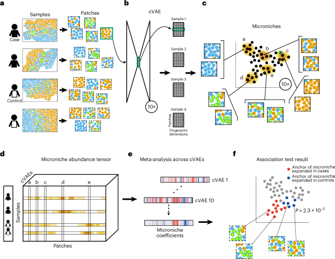
The foundational unit of VIMA’s analysis is the patch fingerprint, which is a compact numerical representation of a small tissue region learned by a variational autoencoder. Each tissue patch, typically measuring 40 by 40 pixels (corresponding to approximately 400 by 400 micrometers), is converted into a vector in a learned latent space. These fingerprints serve a dual purpose: they enable quantitative comparison between patches and preserve the biological information content of the original tissue measurements while discarding noise and technical artifacts.
The variational autoencoders used to generate these fingerprints are trained to reconstruct the input patches from their compressed representations. During training, the models learn to encode biologically meaningful variation while being incentivized to remove sample-specific information that would otherwise compromise cross-sample comparisons. This is achieved through the incorporation of sample-level covariates directly into the network architecture, ensuring that the learned representations are balanced across different biological conditions.
### Microniches
A microniche is defined as a small set of tissue patches from multiple samples that exhibit high biological similarity to one another. Rather than relying on discrete cluster labels, VIMA constructs a continuous measure of patch membership in each microniche using random walks on nearest-neighbor graphs. For each patch in the dataset and each trained autoencoder, a microniche is anchored at that patch, and the degree to which other patches belong to it is determined by the probability that a random walker starting from a given patch will arrive at the anchor patch after a specified number of steps.
This random-walk-based definition provides several advantages. It captures local tissue structure in a continuous manner, allows patches to belong partially to multiple microniches, and naturally accommodates the variability inherent in biological samples. The microniche construction is performed independently for each autoencoder, resulting in ten parallel sets of microniches that collectively describe the tissue landscape from complementary perspectives.
## Methodology
### Preprocessing and Quality Control
VIMA’s preprocessing pipeline addresses three critical challenges common in spatial molecular datasets. First, tissue regions are separated from background using modality-specific signal summarization and thresholding strategies. For transcript-based measurements, a minimum transcript count per pixel is applied, while for protein-based measurements, adaptive thresholding methods are used to handle nonspecific background staining.
Second, the dimensionality of the marker space is reduced through a multi-step process that includes log-normalization, spatial smoothing, principal component analysis, and harmonization. This produces a manageable set of meta-markers that capture the dominant sources of biological variation while remaining computationally tractable.
Third, sample-specific and batch-specific artifacts are removed using an established batch correction algorithm applied to the reduced-dimensional representations. This step ensures that downstream analyses reflect genuine biological differences rather than technical confounders.
### Autoencoder Training and Patch Featurization
After preprocessing, tissue patches are extracted from each sample at a resolution of 40 by 40 pixels. Only patches containing sufficient tissue density are retained for analysis. Ten conditional variational autoencoders are then trained in parallel to learn latent representations of these patches.
Each autoencoder is a modified convolutional neural network designed to operate on the small patch dimensions. The conditional design is critical: both the encoder and decoder receive information about sample identity and any additional covariates through a learned embedding that is broadcast across all spatial locations in the patch. This architectural choice ensures that the latent space is structured to maximize cross-sample integration while preserving biological signal.
The training process uses standard practices including held-out validation, learning rate scheduling, and warmup of the variational penalty term. The default configuration balances reconstruction fidelity with latent space semantics, though the framework is flexible enough to accommodate different trade-offs depending on the dataset characteristics.
### Microniche Construction and the Multi-Autoencoder Tensor
Once trained, the autoencoders generate latent embeddings for all retained patches. Microniches are then defined using the nearest-neighbor graph constructed from these embeddings, with membership probabilities computed through random walks that have been calibrated to ensure adequate mixing across samples.
These operations are aggregated into a Multi-Autoencoder Tensor, or MAT, which is a three-dimensional array with dimensions corresponding to samples, patches, and autoencoders. Each entry in the MAT represents the expected fraction of patches from a given sample that would belong to a particular microniche according to a specific autoencoder. This tensor serves as the input for all subsequent statistical analyses, and the software implementation allows for the projection of covariates out of the tensor to isolate biological signals of interest.
### Statistical Association Testing
VIMA implements two complementary levels of statistical testing. The local association test identifies specific microniches whose abundance correlates with a phenotype of interest, such as disease status or treatment group. For each microniche, a meta-analyzed correlation coefficient is computed by aggregating correlations across all ten autoencoders, with each autoencoder’s contribution weighted by the square of its correlation to emphasize models that capture stronger signals.
The global association test assesses whether any microniches across the entire tissue exhibit aggregate association with the phenotype. This test statistic is computed by taking a ratio of fourth to second moments across all patches and autoencoders, providing a summary measure of the total correlation signal present in the data.
Statistical significance is evaluated through permutation testing, where the phenotype labels are shuffled while preserving the structure of multiple samples from the same donor. This preserves the dependence structure inherent in spatial datasets and generates an empirical null distribution against which observed test statistics can be compared. False discovery rates are estimated empirically from the permutation distribution, providing calibrated confidence in the identified associations.
## Validation and Applications
### Simulation Studies
Rigorous simulation studies were conducted to evaluate the calibration, statistical power, and spatial accuracy of VIMA. Using a real spatial transcriptomics dataset from the Seattle Alzheimer’s Disease Brain Cell Atlas, researchers generated null datasets by assigning random case-control labels and confirmed that VIMA’s false positive rates were well-controlled at the nominal significance level.
In non-null simulations, known tissue structures were artificially introduced into case samples at varying abundances, and VIMA was tested on its ability to detect these signals. The framework demonstrated strong power across a range of signal strengths and accurately localized the spatially associated tissue regions. An area under the receiver operating characteristic curve was used to quantify spatial accuracy, with VIMA achieving high discrimination performance even when signals were subtle.
### Real-World Dataset Analyses
VIMA was applied to three heterogeneous spatial datasets spanning different tissues, modalities, and biological contexts. In rheumatoid arthritis synovial biopsies profiled with immunofluorescence microscopy, the method identified tissue microniches associated with stromal versus immune tissue states, revealing marker expression patterns that distinguished these compartments. The analysis showed that VIMA’s microniche framework could recover known tissue organization while also uncovering novel associations.
In ulcerative colitis colonic biopsies profiled with multiplexed immunofluorescence, VIMA identified microniches significantly associated with disease status and further explored treatment-related signatures. By filtering for disease-associated patches and re-analyzing them for treatment associations, the framework revealed tissue patterns associated with both current and past TNF inhibitor use, demonstrating its ability to capture multiple layers of biological signal within the same dataset.
In postmortem brain tissue from dementia patients profiled with MERFISH spatial transcriptomics, VIMA detected microniches associated with dementia status and mapped these to specific cortical layers. The analysis revealed enrichment of specific cell types in dementia-associated microniches and validated findings through complementary non-spatial analyses, demonstrating concordance between spatial and bulk approaches.
### Benchmarking Against Existing Methods
VIMA was systematically compared against a suite of existing tissue annotation methods including CellCharter, STAGATE, UTAG, CANVAS, and TissueMosaic, as well as simpler baseline approaches that use patch-level averages or cell-type abundances. Across all three datasets, VIMA demonstrated competitive or superior performance in identifying case-control associated tissue features, as measured by global and local significance testing.
The integration properties of VIMA were also assessed by examining how well each method’s embeddings preserved sample identity in nearest-neighbor graphs. VIMA’s multi-autoencoder approach consistently achieved strong sample integration, indicating that the latent representations effectively removed technical variation while retaining biological signal. Ablation studies further confirmed that the conditional autoencoder architecture, the microniche framework, and the ResNet backbone each contributed independently to the method’s performance.
## Frequently Asked Questions
### What types of spatial data can VIMA analyze?
VIMA is designed to be modality-agnostic and can analyze any spatial molecular data that has been rasterized into a pixel grid with measurements for multiple markers or genes. The method has been demonstrated on protein-based measurements from immunofluorescence and CODEX imaging, as well as transcript-based measurements from MERFISH and similar technologies. The preprocessing step automatically adapts its signal summarization strategy depending on whether the data represents transcripts or proteins.
### How does VIMA handle batch effects?
Batch effects are addressed at multiple stages of the VIMA pipeline. During preprocessing, the Harmony algorithm is applied to the reduced-dimensional meta-marker representations to remove sample-specific and batch-specific variation. Additionally, the conditional autoencoder architecture incorporates sample identity embeddings that help the model learn representations that are invariant to batch while retaining biological signal.
### What is the computational cost of running VIMA?
The computational requirements depend on dataset size, number of markers, and the number of patches. Training ten autoencoders in parallel is more efficient than training them sequentially, as backpropagation and data loading contribute significant overhead. For the datasets analyzed in the method’s validation, training times are on the order of hours rather than days. The microniche construction and statistical testing steps are optimized for sparse matrix operations, making them scalable to large numbers of patches.
### How does VIMA differ from cell-type-based approaches?
Unlike methods that require cell segmentation and cell-type annotation as a prerequisite, VIMA operates directly on pixel-level measurements and learns tissue representations without relying on discrete cell boundaries. This makes it applicable to datasets where cell segmentation is challenging or unavailable, such as certain immunofluorescence experiments with irregular tissue morphology. Furthermore, the microniche framework captures continuous tissue gradients and subtle spatial patterns that may not correspond neatly to canonical cell types.
### Can VIMA be applied to datasets with covariates beyond case-control status?
Yes, VIMA’s statistical framework can accommodate any sample-level phenotype or covariate. The autoencoder architecture can incorporate additional covariates beyond sample identity, and the association testing can be performed with any variable of interest. The software implementation also supports projection of specified covariates out of the microniche abundances, allowing researchers to control for potential confounders.
### What parameters need to be specified by the user?
VIMA includes sensible defaults for all key parameters, including the patch size, the number of autoencoders and their latent dimensionality, the tissue density threshold for patch inclusion, and the number of meta-markers. Users can adjust these defaults based on their specific dataset characteristics, and the authors recommend increasing the variational penalty parameter if patches are not sufficiently integrated across samples.
## Discussion
The VIMA framework represents a significant advance in the analysis of spatial molecular data by combining the representational power of deep learning with rigorous statistical inference. Its multi-autoencoder design provides robustness against model-specific biases and captures diverse aspects of tissue organization that might be missed by single-model approaches. The microniche concept offers a flexible, continuous description of tissue neighborhoods that goes beyond traditional clustering-based tissue annotation.
One of the most compelling aspects of VIMA is its ability to operate without requiring cell segmentation or prior knowledge of cell types, making it broadly applicable across tissue types and experimental modalities. This is particularly valuable in fields such as pathology and drug development, where tissue morphology can be highly variable and where segmentation may be unreliable or impractical.
The method’s comprehensive validation strategy, including null and non-null simulations alongside benchmarking on diverse real-world datasets, provides strong evidence for its reliability and utility. The ablation studies confirm that each component of the method contributes meaningfully to its overall performance, and the integration analysis demonstrates that VIMA’s representations effectively balance sample mixing with biological signal preservation.
## Limitations and Future Directions
While VIMA has demonstrated strong performance across multiple datasets and modalities, there are areas where further development could extend its capabilities. The current implementation uses fixed patch sizes, which may not be optimal for all tissue types or spatial scales. Future versions could incorporate adaptive patch sizing or multi-scale analysis to capture tissue architecture at varying resolutions.
The framework currently assumes that the 40 by 40 pixel patch size is appropriate for the biological questions being asked, but finer spatial resolution could reveal subcellular patterns that are currently missed. Additionally, the method’s reliance on variational autoencoders means that the quality of learned representations depends on appropriate tuning of the trade-off between reconstruction and latent space regularization, though the authors found this to be robust across datasets.
Extensions to time-series or longitudinal spatial datasets, where the same tissue region is profiled at multiple time points, could further enhance the method’s applicability to dynamic biological processes. Integration with other spatial analysis tools and compatibility with emerging spatial modalities would also broaden VIMA’s impact.
## Conclusion
VIMA provides a comprehensive, statistically rigorous framework for analyzing spatial molecular tissue data with the goal of identifying biologically meaningful tissue neighborhoods associated with disease or other phenotypes of interest. By combining variational autoencoders for unsupervised feature learning with a microniche-based framework for tissue representation and meta-analytic statistical testing, the method offers a powerful alternative to both manual annotation approaches and simpler automated pipelines. Its demonstrated performance across diverse tissues, modalities, and biological contexts positions VIMA as a valuable tool for the growing field of spatial biology and precision medicine.
Thank you for reading
