



# Measuring Intervention Effects When Randomized Trials Aren’t Possible: A Practical Guide to Interrupted Time Series Analysis and Automated Multi-Agent Systems
## Introduction
Imagine this scenario: your company launches a brand new checkout process. The hypothesis is straightforward—a streamlined three-step checkout will drive more purchases and revenue than the previous one-step flow. You recommend running an A/B test to measure the effect and validate the decision scientifically. However, stakeholders push back, the launch goes ahead without a properly controlled experiment, and now everyone wants to know: “Did it actually work?”
This situation is more common than most data professionals care to admit. When randomization isn’t feasible, control groups don’t exist, and the organization isn’t large enough to build credible comparison regions, what tools do you have left? This is where Interrupted Time Series Analysis (ITSA) enters the picture—a powerful quasi-experimental technique that builds its counterfactual from your own historical data.
This article explores what ITSA is, why it matters for digital business measurement, how a multi-agent artificial intelligence system can automate and standardize the analysis, and what limitations you should understand before trusting the results.
—
## Understanding Interrupted Time Series Analysis
### The Problem with Simple Before-and-After Comparisons
The most intuitive approach to measuring an intervention’s effect is comparing what happened before with what happened after. In practice, this usually means taking the average of the pre-intervention period and comparing it to the average of the post-intervention period, then calling the difference the “lift.”
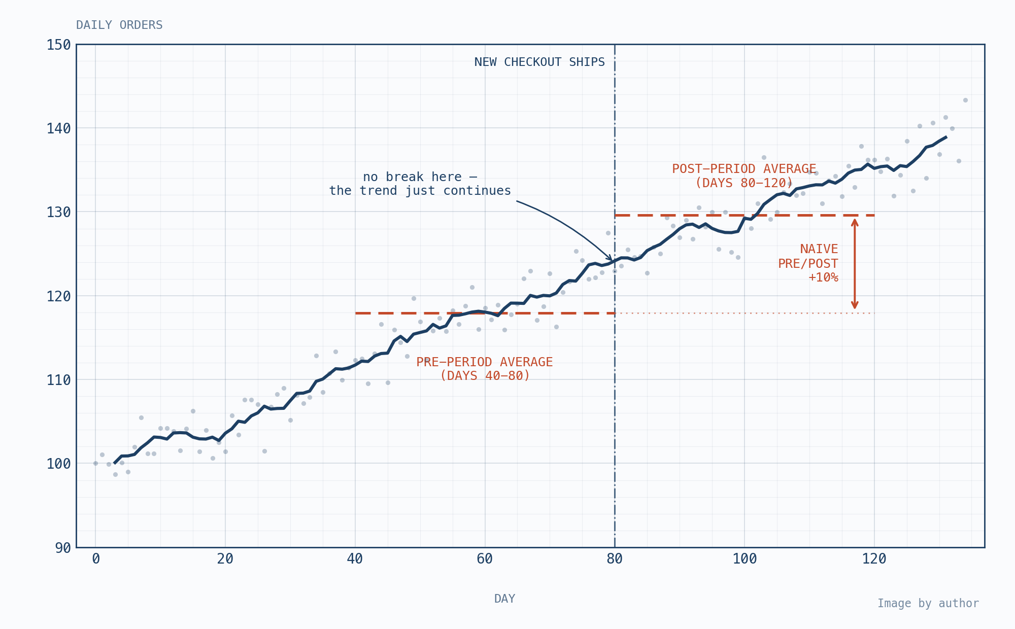
This approach fails in subtle but critical ways. Consider a scenario where daily orders have been climbing steadily from about 100 to 140 over a span of 130 days. A new checkout process launches on day 80, and the upward trend simply continues. If you compare the pre-period average (days 40–80) with the post-period average (days 80–120), you might see a 10% increase and conclude the new checkout drove it. In reality, the trend was already moving upward, and the intervention had no additional effect at all.
The fundamental issue is that comparing averages ignores pre-existing trends, seasonality, and autocorrelation while treating every change after the intervention date as causal. What’s needed instead is a method that constructs a counterfactual—a projection of what would have happened had the intervention never occurred—and then measures the gap between reality and that projection.
### How ITSA Constructs a Counterfactual
Interrupted Time Series Analysis takes a fundamentally different approach. Rather than comparing two averages, it uses the outcome’s own pre-intervention trajectory to estimate what would have happened after the intervention in its absence. In its most common form, a segmented regression model estimates the baseline level and the pre-existing trend, then projects that trajectory forward into the post-intervention period.
The intervention effect isn’t the difference between post-intervention and pre-intervention averages. It’s the difference between what actually happened and what the model projected would have happened. Formally, the effect at any given time is the observed outcome minus the estimated counterfactual: τ_t = Y_t(1) − Ŷ_t(0).
In one illustrative example, a steady upward trend continues unchanged after a new process launches. The pre-intervention trend gets projected forward as a dashed line with an uncertainty band—representing what would have happened without the change. When the observed data points fall within that band, the estimated effect is essentially zero. The new process didn’t move the needle; the underlying trend did.
This counterfactual construction is what separates ITSA from naive pre/post comparisons and makes it valuable for situations where randomized control trials and traditional quasi-experimental methods aren’t viable.
### The Core Assumptions You Must Understand
ITSA rests on ten important assumptions that every practitioner should know before applying it:
**1. Counterfactual Continuity:** Without the intervention, the pre-intervention trend would have continued unchanged. This is the assumption that carries all the analytical weight and is fundamentally untestable—you never observe the world without the intervention. It connects directly to the fundamental problem of causal inference.
**2. A Clear Intervention Point:** You need a well-defined onset date. The timing must be unambiguous.
**3. No Co-Interventions or Concurrent Shocks:** No other policy changes, campaigns, or external events should occur around the intervention date that could explain the observed interruption. This is known as the history threat.
**4. No Anticipation:** The intervention should not affect behavior during the pre-intervention period. If people change their actions before the official launch, the baseline is already contaminated.
**5. Smooth Time-Varying Confounders:** Any confounders that change over time must evolve smoothly, remaining distinguishable from the sharp jump introduced by the intervention. An abrupt confounder masquerades as an intervention effect.
**6. Controlled Seasonality and Cycles:** Day-of-week patterns, monthly cycles, and recurring campaigns must be accounted for in the model.
**7. Sufficient Observations:** You need enough equally-spaced data points both before and after the intervention. A common rule of thumb is at least eight observations per segment. Without adequate data, the minimum detectable effect rises above the real effect, and you’ll fail to find it.
**8. Proper Handling of Autocorrelation:** Time-series errors are serially correlated. Ignoring this produces miscalibrated standard errors and confidence intervals that are too narrow or too wide.
**9. Consistent Outcome Measurement:** The metric’s definition and collection methods must remain stable across both the pre-intervention and post-intervention periods. Changing measurement protocols mid-stream invalidates the comparison.
**10. Valid Regression Model Assumptions:** The underlying regression model’s own assumptions—linearity, independence of errors (after accounting for autocorrelation), homoscedasticity, and distributional properties—must hold.
When these assumptions line up, ITSA becomes not just a fallback option but often the best tool available for single-group intervention analysis.
### When ITSA Is the Right Choice
ITSA shines when three conditions converge simultaneously:
**You couldn’t randomize.** The change was deployed to everyone at once—perhaps a new checkout flow, a pricing change, or an infrastructure migration. There is no untreated group to compare against.
**You have no credible control group.** There’s no parallel market, region, or product line that behaved like yours but never received the change. This rules out difference-in-differences and synthetic control methods, both of which require comparison units. ITSA is the single-group design because it builds the counterfactual from your own history rather than from an external comparison.
**You have a clean time series.** One consistently measured outcome, collected at regular intervals, with sufficient observations both before and after a clearly dated intervention point.
It’s important to understand that ITSA is better understood as a research design than a single estimation technique. It should never be selected merely because you have a time series and an intervention date. If the intervention timing is ambiguous, the pre-intervention period is already contaminated by another relevant event, or the series provides too little temporal support, no amount of statistical sophistication can rescue the identification strategy.
—
## The Multi-Agent System Approach to Automating ITSA
### Why Automation Matters
Organizations that regularly need to measure intervention effects face a practical problem: manual ITSA analysis is time-intensive. What once took data teams six hours per analysis—loading data, running diagnostics, selecting models, interpreting outputs, and building reports—becomes a bottleneck when stakeholders need answers quickly.
Early efforts to streamline this process involved scripted Python pipelines that could automatically determine the best statistical approach based on input parameters. These tools reduced analysis time from six hours to thirty minutes and standardized the methodology across teams. However, they reached a point of diminishing returns: adding more visual graphs, flexibility, and statistical approaches required increasingly complex parameterization and deep statistical knowledge with each iteration.
This is where multi-agent artificial intelligence systems offer a fundamentally different path forward.
### How a Multi-Agent Architecture Works
The core idea behind an AI-powered ITSA system is to separate the statistical computation from the reasoning and communication layers using multiple specialized agents.
The first agent acts as a quantitative analyst. It follows a prescribed sequence of steps—loading data, checking stationarity, testing for seasonality, examining autocorrelation, and so on—before selecting the primary estimation approach that fits what those diagnostics reveal. The analyst agent doesn’t compute a single number itself. Instead, it calls twelve deterministic Python tools that perform the actual calculations using libraries like statsmodels, scipy, and pandas.
Why keep the tools deterministic? Because the same input must always produce the same output, regardless of whether an AI model is involved. The model’s role is to reason about the outputs, not to generate the outputs themselves. Choosing the right estimator for a non-stationary count series with weekly seasonality is a judgment call. Computing its coefficients is arithmetic—and arithmetic is the last thing you want an AI model doing.
The analyst finishes with a structured summary: the estimated effect and its uncertainty, any warnings that apply, a confidence level, and a recommended action drawn from a closed vocabulary (such as “uplift detected and statistically significant,” “no significant effect found,” or “recommend stopping the intervention”). This summary takes the form of a schema-validated JSON file—the only contract between agents.
The second agent, called the storyteller, takes that structured JSON and translates it into a stakeholder-facing report. It has its own identity, its own base prompt, and its own set of tools focused on visualization and presentation rather than statistics. It never sees the raw dataframe, never runs models, and cannot recompute effects or upgrade a “no significant effect” finding into a positive one. It receives only the committed output from the analyst agent and builds the narrative around it.
This separation of concerns is deliberate. The storyteller cannot invent anything because none of the underlying numbers are within its reach. Everything it communicates must trace back to what the analyst agent explicitly committed to in writing.
—
## Encoding Exposure Share for Real-World Interventions
### Why Binary Intervention Coding Falls Short
Textbook ITSA treats the intervention as a simple 0/1 indicator: before the intervention date, the variable is zero; after it, the variable is one. This assumes the treatment applies fully and instantly to the entire population from day one.
Real business interventions rarely behave this way. A new checkout process might initially go to 20% of traffic and gradually expand to everyone over two weeks. A mobile app feature might roll out market by market across six weeks. A marketing campaign might burn bright for five days and then stop. A binary dummy variable tells the model that the entire audience was treated from day one, when in reality most of the audience wasn’t. This fiction gets baked into every coefficient estimated afterward.
### The Exposure Share Concept
The solution is to replace the binary indicator with an exposure share—a value between 0 and 1 that represents what proportion of the audience was actually treated on any given day. The intervention then enters the regression model as this continuous variable rather than as a step function.
Four common exposure shapes can be encoded:
**Step:** The classic indicator, switching from 0 to 1 at the intervention date and staying at 1 permanently. This is appropriate when the treatment applies to everyone from the moment it launches.
**Ramp:** The exposure share interpolates linearly from 0 to 1 across a rollout window, then holds at 1. This models staged rollouts where a percentage of users are migrated each day.
**Pulse:** The exposure is 1 for the duration of a burst and 0 on either side. This captures campaigns or interventions that run for a fixed period and then stop.
**Decay:** The exposure declines over time following an exponential decay curve, with a half-life parameter controlling how quickly the effect fades. This is appropriate for temporary interventions whose impact diminishes after the active period ends.
The exposure share enters the design matrix twice in the model—once on its own for the level change and once multiplied by the post-intervention time term for the slope change. Coefficients are then interpreted as the level change and slope change per unit of exposure, rather than as raw absolute changes.
### Why This Matters in Practice
Consider a staged market rollout scenario. If you code the intervention as a step on the first launch date, you’re telling the model the entire audience was treated from day one. The early post-intervention days—when most users were still untreated—pull the estimate toward zero. A genuine effect gets diluted into what appears to be “no significant change.”
The alternative is to move the intervention date to when the rollout completed and discard the weeks in between. This trades one bias for the loss of half your post-intervention data. With an exposure share, you don’t have to choose. Every day enters the model weighted by how much of the audience had actually been reached by then.
The deeper advantage is that the intensity of treatment is often something you already know from project documentation—traffic allocation percentages, launch calendars, campaign start and end dates. Encoding this information costs no extra data collection; it simply stops you from discarding knowledge you already possess.
One important caveat: the model assumes the treatment effect is linear in exposure. If 40% of the audience reached produces 40% of the effect, great. But if the users reached early respond differently from those reached later—due to novelty effects or compositional differences—the exposure share conflates intensity with composition, and the coefficient can’t distinguish between them.
—
## Diagnostic Checks That Encode Assumptions
### From Prompt Checklists to Deterministic Validation
One of the most critical design decisions in building an automated ITSA system is ensuring that the core assumptions are verified computationally rather than left to chance. A prompt can serve as a wishlist, but what you actually need is a checklist that runs deterministically before any AI reasoning begins.
The system computes the shape of the problem in plain Python before the agent ever gets to interpret anything. Three diagnostic values are particularly telling:
**Pre-trend R-squared** tells you whether the series was already trending before the intervention. A low value means the pre-intervention period is relatively flat, giving the extrapolated counterfactual more confidence. A high value signals a strong existing trend, which means the counterfactual projection carries more weight and more risk.
**Pre-end Excursion Z-score** measures what happened right before the intervention. It detects whether the final observations of the pre-period were abnormal—perhaps showing an unexpected spike or dip that suggests the world was already moving before the intervention officially began.
**Pre-both-Halves Significance** checks whether the trend holds consistently across the entire pre-period or whether it’s driven by one particular stretch of time. If the slope is significant in the first half but not the second, or vice versa, the stability of the pre-intervention trend is questionable.
### Handling Ambiguous Statistical Results
Statistical tests sometimes disagree with each other. A common scenario is the Augmented Dickey-Fuller test failing to reject a unit root while the KPSS test also fails to reject stationarity. Taken together, this is inconclusive rather than a clean verdict.
Rather than asking the AI model to resolve the ambiguity—a stochastic output that could change with each run—the system applies a fixed conservative routing rule. In the case of disagreement between stationarity tests, the series is treated as non-stationary for model selection purposes, while both results and the conflict are recorded. This routing decision is repeatable, even when the statistical evidence remains genuinely ambiguous.
### Autocorrelation Detection as a Routing Signal
Similarly, autocorrelation is detected through formal tests—Durbin-Watson statistics and Ljung-Box tests at multiple lags—rather than flagged in a prompt. When Durbin-Watson falls below 1.5 and Ljung-Box p-values are significant at lags 1, 7, 14, and 30, the system routes toward HAC (heteroskedasticity and autocorrelation consistent) standard errors. This single deterministic flag drives the estimator choice downstream.
The key principle throughout this approach is that diagnostics tied to the assumptions of the analysis are computed deterministically, not delegated to a stochastic output from an AI model. The model is used for reasoning—deciding what to run and what the results mean—while the tools guarantee that the same inputs always produce the same numerical outputs.
—
## Evaluating Trustworthiness: How Do We Know It Works?
### The Benchmarking Framework
To assess whether an automated ITSA system produces reliable results, a rigorous benchmarking approach is essential. The evaluation involves running the system against more than 150 different datasets—spanning real-world cases, semi-synthetic scenarios built on actual data, and fully synthetic cases with known ground truths.
For each scenario, the ground truth includes the injected effect size (if any), whether detection should be expected, the direction of the effect, and which warnings the system should raise. Every output is then compared against this known truth.
### Two Layers of Evaluation
Each run is scored through two distinct layers:
**Deterministic checks (40% of the score)** validate the output against the ground truth directly. Did the system detect an effect when one was expected? Did it avoid claiming detection when no effect was present? Did it get the direction correct? Was the estimated magnitude within 30% of the true effect? Did it classify stationarity correctly? Did it avoid inappropriate statistical tests? And crucially, did it raise warnings for the planted traps embedded in each scenario?
**An LLM-based judge (60% of the score)** evaluates the quality of the written narrative across five dimensions: diagnostic quality, model selection rationale, interpretation of results, honesty about caveats and limitations, and clarity of business communication. This carries more weight because the system isn’t only expected to calculate the right result—it also needs to reason about it and communicate it in ways that support real business decisions.
### Learning from Benchmark Drops
The benchmarking process reveals important patterns about where improvements come from. Early iterations tend to show gains from fixing arithmetic bugs—boolean values serialized incorrectly, seasonality gates triggering at the wrong thresholds, structural-break rules firing on noise. Later improvements come from statistical refinements. The final stretch of gains is often semantic rather than technical: normalizing the output vocabulary so that what the system says matches what evaluators expect to hear. Sometimes, it even means fixing the evaluation itself—scenarios that demanded detection of effects below the minimum detectable threshold for the series, or scenarios where a true effect wasn’t detectable given the data’s power.
The overarching lesson is straightforward: iteration by iteration, improvements accumulate. Arithmetic problems get resolved first, then statistical ones, and the final improvements are almost entirely about semantic alignment between what the system reports and what stakeholders need to hear.
—
## Limitations: What ITSA Can’t Fix—and Why It’s Still Worth Using
### The Two Structural Challenges
Honesty about limitations is essential when recommending any analytical method. ITSA has two structural challenges that practitioners should understand.
**The counterfactual continuity problem.** The entire design leans on the pre-trend having enough predictive strength to serve as the counterfactual. When the true counterfactual bends—say, an underlying growth trend accelerates after the intervention—the linear extrapolation of the pre-intervention trend doesn’t fail loudly. Instead, it quietly overestimates the effect on every post-intervention day. The gap between the observed data and the assumed counterfactual becomes larger than the true intervention effect.
**The no-control-group vulnerability.** Because a single-group ITSA design has no control group, the projected pre-intervention trajectory must serve double duty as both the baseline and the counterfactual. While covariates can adjust for observed time-varying confounders and improve counterfactual prediction, they cannot rule out unobserved shocks that coincide with the intervention. This is precisely why difference-in-differences or synthetic control methods can be more defensible when a credible comparison series is available.
### Checks That Still Need to Be Built
There’s also a family of diagnostic checks that aren’t yet standard in automated systems. The first is the in-time placebo test: re-running the analysis with a fake intervention date somewhere in the pre-period where nothing happened. If the pipeline reports an effect there, the design is leaking—saying more about whether you can trust any result than any single diagnostic could.
The second is sensitivity analysis: how much does the estimate move if the intervention date shifts by a few days, or if the declared exposure shape is wrong? Currently, the shape and half-life are declared once before the analysis begins, which is the minimum defense against tuning the geometry until the p-value cooperates. But declaring a parameter isn’t the same as knowing how much the answer depends on it.
### Why These Limitations Don’t Diminish the Value
Despite these limitations, ITSA remains an enormously valuable method—and transforming it into an accessible AI product creates outsized organizational value. Counterfactual reasoning has historically lived behind a wall of specialized data scientists. Now, someone in marketing or product can upload a CSV, declare an intervention date, and receive an analysis with a counterfactual projection, uncertainty estimates, and warnings that until recently required a specialist most companies don’t employ.
The real strategic value lies in what ITSA teaches organizations to think: in counterfactuals. One line for what happened, one line for what would have happened, and the effect is the gap between them. Once an organization learns to think this way, it has earned the credibility to eventually adopt more complex and better-identified experimental designs.
—
## Frequently Asked Questions
**Q: How is ITSA different from a simple before-and-after comparison?**
A: A before-and-after comparison looks at the difference between two averages—one from the period before the intervention and one from after. ITSA goes further by fitting a model to the pre-intervention trend and projecting it forward as a counterfactual. The effect is the gap between what actually happened and what the model projected would have happened, not the gap between two period averages. This approach accounts for pre-existing trends, seasonality, and autocorrelation rather than ignoring them.
**Q: When should I choose ITSA over difference-in-differences or synthetic control?**
A: Choose ITSA when you have no untreated comparison group available. Difference-in-differences requires parallel trends across at least two groups, and synthetic control needs a weighted combination of control units that resemble the treated unit. If your organization ran a company-wide change—like a pricing update or checkout redesign—with no regions, product lines, or user segments left untreated, ITSA is often the best single-group option because it builds its counterfactual from your own historical data.
**Q: What does “exposure share” mean in practice?**
A: Exposure share replaces the traditional binary 0/1 intervention indicator with a continuous value between 0 and 1 that represents the proportion of the audience actually treated on any given day. For a gradual rollout starting at 0% and reaching 100% over two weeks, the exposure share on day three might be 0.25, on day seven might be 0.70, and so on. This prevents the model from treating untreated early-period users as if they experienced the full intervention.
**Q: Why use multiple AI agents instead of one?**
A: Separating the system into a quantitative analyst agent and a storytelling agent creates clear boundaries. The analyst handles computation and reasoning about statistical outputs using deterministic tools that always produce the same results. The storyteller handles communication and visualization using only the analyst’s structured JSON output—never raw data, never model computation. This separation prevents the storytelling agent from inventing or distorting results while allowing each agent to specialize in what it does best.
**Q: How does the system ensure that statistical diagnostics are trustworthy?**
A: The system computes key diagnostics—stationarity tests, autocorrelation checks, pre-trend stability metrics—deterministically in Python before any AI reasoning begins. These values are recorded and used to route model selection and flag warnings. The AI agent then reasons about these pre-computed diagnostics rather than generating its own statistical outputs, which would be stochastic and potentially inconsistent.
**Q: What happens when statistical tests disagree?**
A: When tests like the Augmented Dickey-Fuller and KPSS give conflicting results about stationarity, the system applies a fixed conservative routing rule rather than relying on the AI model to interpret the ambiguity. In this case, it defaults to treating the series as non-stationary while recording both test results and the conflict. This ensures the routing decision is repeatable and transparent, even when the underlying statistical evidence is genuinely ambiguous.
**Q: How accurate are the automated results compared to manual analysis by a statistical expert?**
A: Benchmarking against ground truth across hundreds of scenarios shows that after iterative refinement, automated systems can achieve accuracy scores above 98% on synthetic data and above 99% on well-structured scenarios. Performance is lower on real-world data with unusual patterns (around 67–99% depending on complexity), but the system’s honesty about uncertainty and its ability to flag when detection is unreliable—rather than producing misleadingly precise but wrong results—is a key design strength.
**Q: Can ITSA tell me with certainty whether my intervention worked?**
A: No method can provide certainty when the assumptions don’t hold. ITSA provides an estimated effect with uncertainty bounds and warnings about assumption violations. If the pre-intervention trend is weak, if there were concurrent events around the intervention date, or if the data contains too few observations, the system should flag these concerns rather than produce a confidently wrong answer. The value is in making the uncertainty visible and in providing a counterfactual framing that goes beyond a simple average comparison.
—
## Conclusion
Interrupted Time Series Analysis fills a critical gap in the measurement toolkit. When randomized experiments aren’t possible, when control groups don’t exist, and when organizations need answers about intervention effects without months of specialized statistical work, ITSA provides a principled framework for estimating what changed, by how much, and how confident we can be in that estimate.
The evolution from manual notebook analysis to scripted pipelines to multi-agent AI systems represents more than a productivity improvement—it represents a shift in who can do causal inference. When the analytical machinery is automated and the assumptions are checked deterministically, the barrier to running credible intervention analysis drops dramatically. Marketing teams, product managers, and business stakeholders can now access counterfactual reasoning that was previously confined to specialist data scientists.
However, tools are only as good as the understanding with which they’re wielded. ITSA’s reliance on counterfactual continuity, its vulnerability to unobserved confounders, and the importance of clean time series data mean that it requires thoughtful application. The most valuable output may not be the point estimate of the effect itself but the disciplined thinking the process encourages: about what happened, what would have happened, and what the gap between them actually tells us.
As organizations continue to adopt AI-powered analytical tools, the architecture described here—deterministic tools for computation, structured contracts between agents, and LLMs reserved for reasoning and communication—offers a template for building safe, transparent, and trustworthy data products.
—
Thank you for reading
