



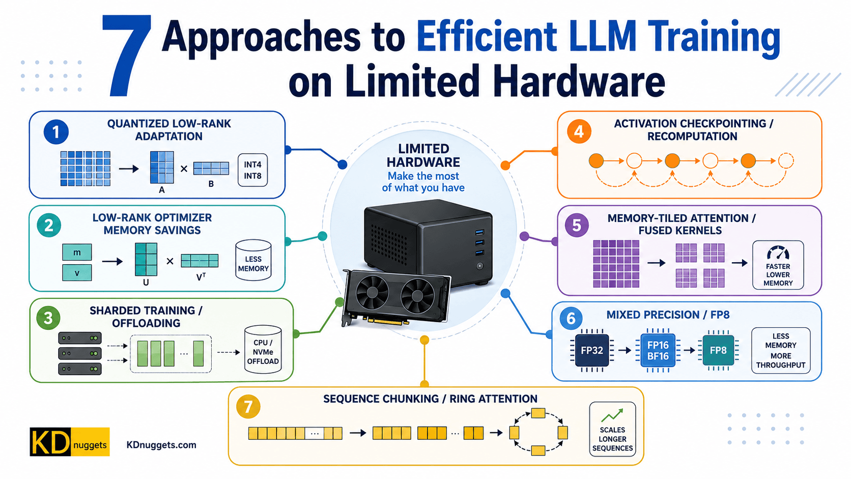
Training large language models is often portrayed as an enterprise-only endeavor requiring massive data center clusters. While scaling laws suggest that pre-training multi-billion parameter models demands clusters of H100s connected by ultra-fast InfiniBand, practical engineering teams frequently operate under strict budget and hardware limitations. Many professionals work with localized setups—dual or quad workstation GPUs like the RTX 4090, A10G, or L40S—constrained by consumer-tier PCIe bandwidth and strict VRAM ceilings of 24 GB to 48 GB per device.
Standard 16-bit training with typical AdamW optimizers will immediately hit a wall. A 7-billion parameter model alone requires 14 GB of VRAM just to store static weights. Add the optimizer states needed for AdamW (which store first and second moment estimates at 8 bytes per parameter) and backward-pass gradients, and the memory footprint explodes, causing an out-of-memory error before a single training step completes. To succeed on constrained hardware, engineers must distinguish between static memory overhead (weights and optimizer states) and dynamic transient memory overhead (intermediate activation maps), while identifying whether a bottleneck is compute-bound or memory-bound.
Here are seven effective approaches to training large models on limited hardware.
**1. Low-Rank Quantization (QLoRA and DoRA)**
The core idea is to freeze the base model weights in a compressed 4-bit representation while injecting trainable, full-precision low-rank matrices into key layers. By quantizing weights into a 4-bit NormalFloat format and applying double quantization—compressing the quantization constants themselves—model footprints shrink dramatically. During training, base weights are dynamically dequantized into BF16 for computation, combined with the low-rank adapter updates, and discarded from cache.
Weight-Decomposed Low-Rank Adaptation (DoRA) extends this by separating the magnitude and directional components of the weights to mirror full fine-tuning trajectories. However, on-the-fly dequantization introduces compute overhead that can degrade training throughput by 20% to 35%. Additionally, merging adapter weights back into the base model for production serving requires dequantizing the base to 16-bit, which can introduce precision loss. This approach is ideal for fine-tuning 7B to 70B parameter models on single or dual consumer-grade 24 GB GPUs.
**2. Gradient Space Optimization (GaLore)**
Unlike parameter-efficient methods that freeze layers, GaLore enables full-parameter learning while drastically reducing memory usage. Standard optimizers track two states per parameter, consuming 8 bytes per parameter. GaLore projects high-dimensional gradient matrices into a compact low-rank subspace, tracking momentum and variance only for the compressed projection rather than the full tensor. These projections are updated periodically rather than every iteration to amortize the computational cost of the decomposition.
The trade-off is that periodic Singular Value Decomposition causes step-latency spikes. Furthermore, selecting the wrong subspace update frequency or rank cutoff can destabilize the training trajectory, causing sudden loss divergence. This is best suited for full-parameter pre-training or aggressive domain adaptation where simpler parameter-efficient methods fail to capture complex out-of-domain feature distributions.
**3. Sharded Data Parallelism with Host Memory Offloading**
Also known as ZeRO-Stage 3 or Full Sharded Data Parallelism, this strategy distributes optimizer states, gradients, and model parameters across all available GPUs and system host RAM. During the forward pass, a collective communication operation reconstructs layer weights just in time for computation, then deallocates them. In offload modes, inactive parameter shards and optimizer states reside in system RAM, streaming across the PCIe bus only when needed.
The major drawback on consumer hardware is I/O bottlenecking. When a GPU finishes its computation before the host-to-device tensor transfers complete, the streaming multiprocessors sit idle, dropping compute utilization. PCIe bandwidth contention can also starve data loader processes, creating a severe pipeline stall. Use this technique when scaling models whose parameter count exceeds the total aggregate VRAM of a multi-GPU node.
**4. Selective Activation Checkpointing**
During a standard backward pass, the system must retain every intermediate activation tensor generated in the forward pass. Selective activation checkpointing flips this paradigm by discarding memory-heavy but compute-cheap intermediate tensors (like activation functions and layer norms) and recalculating them on the fly during the backward pass from the nearest retained boundary.
The downside is a roughly 30% increase in total computational operations. If implemented without careful profiling, frequent memory deallocations and reallocations can cause severe memory fragmentation, triggering out-of-memory errors even when overall VRAM usage appears below the hardware limit. This strategy shines when training with long context windows, where activation memory scales linearly or quadratically and dwarfs static weight allocations.
**5. Memory-Tiled Kernels (FlashAttention-2)**
Standard attention mechanisms materialize a massive N x N attention matrix in high-bandwidth memory, creating excessive read/write traffic. Memory-tiled kernels restructure this computation so that Query, Key, and Value matrices are processed in blocks that fit entirely within the GPU’s fast on-chip SRAM. Softmax normalization is computed incrementally without ever writing the full attention matrix to global memory. Fused kernels further minimize transfers by combining normalization, bias additions, and activations into single operations.
The catch is tight coupling to specific GPU microarchitectures and compute capabilities. Custom kernels can silently fallback to slower native operations or trigger precision underflows on unaligned sequences if not carefully compiled. Regardless of hardware scale, tiled attention kernels are a necessity to maximize streaming multiprocessor occupancy and eliminate memory bandwidth bottlenecks.
**6. Mixed-Precision Training with FP8 Formats**
Running tensor contractions using 8-bit floating-point representations cuts memory bandwidth consumption and activation buffer sizes in half compared to 16-bit formats. This utilizes two distinct FP8 representations: E4M3 (emphasizing numerical precision for weights and activations) and E5M2 (emphasizing dynamic range for gradients). Dynamic scaling factors are computed per-tensor at runtime to prevent underflow and overflow before casting values into dedicated FP8 Tensor Cores.
The narrow dynamic range of FP8 is a significant risk; without rigorous delayed-scaling algorithms, gradient vanishing in deeper layers can cause unrecoverable training divergence. Furthermore, FP8 hardware acceleration is restricted to modern microarchitectures like Ada Lovelace or Hopper and newer. This is the go-to approach for training on RTX 4090, L40S, or H100 hardware where FP8 Tensor Cores can double compute throughput.
**7. Ring-Based Sequence Parallelism (RingAttention)**
For ultra-long contexts, fitting the entire sequence on a single device is impossible. RingAttention slices sequences along the temporal dimension and distributes them across multiple devices. Each device computes attention for its local Query and Key/Value blocks, then initiates an asynchronous peer-to-peer ring communication to pass Key/Value blocks to the next device while receiving from the previous one. Compute and communication overlap entirely, removing the need for high-end NVLink meshes.
On standard PCIe or 1GbE/10GbE local networks, communication latency often outpaces compute time for small batch sizes, causing the pipeline to stall at every ring step and wiping out throughput gains. This is highly effective for scaling context windows beyond 32k tokens across distributed setups that lack dedicated high-bandwidth bridging hardware.
**Conclusion**
Training large models on constrained hardware requires a shift in focus from brute-force compute scaling to meticulous memory hierarchy management. By decoupling weight precision, optimizer state tracking, and activation persistence through techniques like low-rank quantization, gradient projection, and memory-tiled kernels, engineering teams can achieve convergence parity with enterprise-scale compute clusters. Long-running training jobs on consumer hardware will inevitably expose hidden failure modes—thermal throttling, driver-specific kernel instabilities, and asynchronous I/O corruption—making continuous metric tracing and automated gradient verification essential for protecting compute time.
**Frequently Asked Questions**
**Q: Why does standard 16-bit training fail immediately on consumer GPUs?**
A: The static memory footprint of a 7B parameter model alone is 14 GB in FP16. When you add 16 bytes per parameter for AdamW optimizer states and 16 bytes for gradients, plus dynamic activation memory, the total VRAM requirement exceeds the 24 GB limit of most consumer GPUs before training even begins.
**Q: What is the primary drawback of using QLoRA for training?**
A: The dynamic process of dequantizing base weights on-the-fly introduces compute overhead that reduces training tokens-per-second by 20% to 35%. Additionally, if you need to merge the trained adapter back into the base model for production serving, you must convert the base weights back to 16-bit, which can compound precision loss.
**Q: When is it appropriate to use RingAttention?**
A: RingAttention is appropriate when you need to scale your training context window beyond 32,000 tokens but do not have access to high-bandwidth NVLink bridges between your GPUs. It allows you to distribute sequence processing across standard network or PCIe links, though its benefits diminish if the network latency exceeds the per-block compute time.
**Q: Why is FlashAttention-2 considered mandatory for modern transformer training?**
A: It restructures attention calculations to operate entirely within the GPU’s fast SRAM rather than the slower high-bandwidth memory (HBM). This eliminates the need to materialize the massive N x N attention matrix, dramatically reducing memory bandwidth pressure and preventing the GPU’s streaming multiprocessors from idling during memory waits.
Thank you for reading
