



# How AI Search Engines Serve Embeddings at Scale: Infrastructure Patterns for Fast Vector Indexing
## Introduction
Building a high-quality AI search product depends on two critical factors: the accuracy of the embedding model itself, and the cost efficiency with which that model can be run across millions of indexed documents. While much attention goes into model architecture and training, the serving layer — the infrastructure that transforms raw queries and documents into dense vector representations — plays an equally decisive role in search quality and latency.
This article explores the infrastructure patterns behind serving embedding models at production scale, covering workload classification, system architecture, scheduling strategies, and GPU optimization techniques that make fast embedding inference possible.
—
## Two Distinct Workloads, One Shared Engine
Embedding serving can be understood as operating across two fundamentally different workloads, each with its own performance priorities.
### Batch Embedding
Batch embedding occurs during index construction or re-indexing. When a search engine crawls new documents or updates its vector database, it must embed large collections of text in bulk. The primary goal here is **throughput maximization** — processing as many documents as possible per unit of time to minimize infrastructure costs. These workloads are typically scheduled during off-peak hours and run on dedicated GPU capacity.
### Online Embedding
Online embedding happens at query time. When a user submits a search query, the system must embed that short text input as quickly as possible to retrieve relevant results. Latency is the dominant constraint here — even a few hundred milliseconds of delay can degrade the user experience. These requests are short (often just a few tokens), making them fundamentally different from full-sequence inference workloads.
### Scoring: The Bridge Between the Two
Between these two extremes sits the ranking phase. After initial vector similarity search retrieves candidate documents, large batches of those documents must be scored and re-ranked. This workload balances both throughput and latency considerations, as ranking models process multiple documents per query to determine the final ordered result set.
—
## Reusing the LLM Stack: A Strategic Decision
A key architectural decision in embedding-serving infrastructure is whether to build a dedicated engine from scratch or to leverage existing components from the language model serving stack.
Embedding models are, at their core, small Transformer architectures. This structural similarity has a profound implication: **batch embedding closely resembles compute-bound prefill operations**, while **online embedding with short token sequences closely resembles memory-bound decode operations**. Because these two workloads map onto the same computational primitives used in large language model serving, teams can reuse prefill and decode kernels rather than duplicating infrastructure.
This approach reduces engineering overhead and allows embedding serving to benefit from the same optimization work — kernel tuning, memory management, and device scheduling — already invested in the LLM pipeline.
—
## The Three-Service Architecture
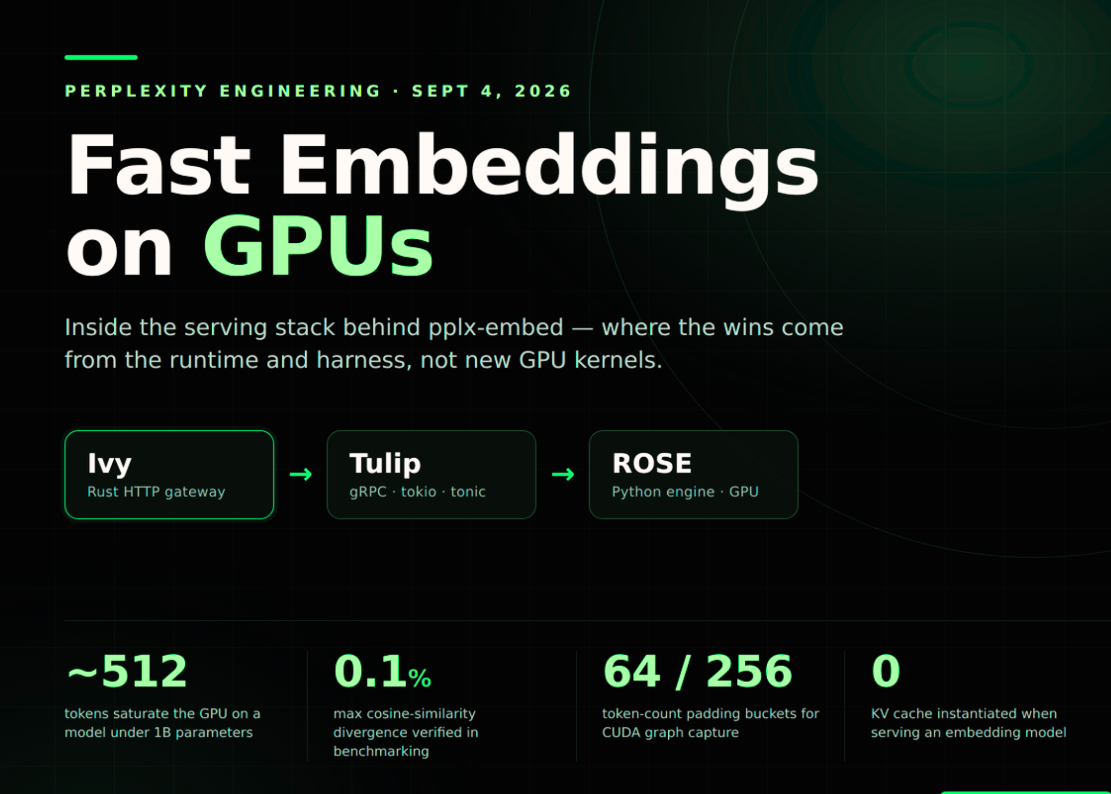
The serving stack is organized into three distinct layers, each written primarily in Rust with the exception of the inference engine itself.
### Layer 1: Ivy — The HTTP Gateway
Ivy functions as the entry point for all embedding requests. Written in Rust, it handles all CPU-side preprocessing:
– **JSON parsing** of incoming HTTP requests
– **Tokenization** using an in-house unigram tokenizer
– **Input templating** to format text for the model
– **Batch splitting** of large requests into smaller, manageable chunks
– **Load balancing** across multiple replicas to correct imbalances caused by variable production payload sizes
Ivy translates these preprocessed requests into a custom gRPC protocol before forwarding them to the next layer. By keeping all CPU-bound work in this gateway, the GPU-bound stages can remain focused on acceleration.
### Layer 2: Tulip — The Inference Server Interface
Tulip is a gRPC server built with Rust, using the `tokio` asynchronous runtime and `tonic` for gRPC communication. It serves as the bridge between the gateway and the actual inference engine:
– **Request scheduling**: Sequences are collected first-come, first-served as they arrive
– **Batch assembly**: Accumulated sequences are packed into batches for GPU dispatch
– **Kernel dispatching**: Batches are sent to the underlying inference engine
A notable design choice is that Tulip’s scheduler remains deliberately simple. It does not implement complex priority queues or sophisticated batching algorithms. This simplicity is justified by empirical measurements specific to small embedding models at the sequence lengths served in production.
### Layer 3: ROSE — The Runtime-Optimized Serving Engine
ROSE is the Python-based inference engine that actually executes the model on the GPU. It provides:
– **Custom CUDA kernels** optimized for embedding operations
– **Model layer definitions** and architecture specifications
– **CUDA graph management** for capturing and replaying GPU workloads
– A **`step()` function** that Tulip calls to execute inference
ROSE does not allocate a KV cache for embedding operations, since embedding models process sequences differently from autoregressive language models. This omission is one of the reasons embedding inference can be made faster and more memory-efficient.
—
## Why the Scheduler Is Deliberately Simple
The first-come, first-served scheduling approach in Tulip works well for embedding models because of a specific characteristic of their computational profile.
For small embedding models at typical sequence lengths, the **linear cost of dense feed-forward layers dominates the quadratic cost of self-attention**. This means that the time to process a batch is roughly proportional to the number of tokens, not the number of sequences.
There is a practical ceiling to this effect. Once a batch **saturates the GPU** — which occurs at approximately **512 tokens on a sub-billion-parameter model** — adding more sequences to the batch yields no additional efficiency gains. The GPU is already fully utilized, and further packing is wasted effort.
This measurement eliminates the need for complex dynamic batching strategies, as the optimal batch size is relatively predictable and bounded.
—
## CUDA Graphs: Eliminating Kernel Launch Overhead
On small batches, the overhead of launching individual GPU kernels from the CPU can outweigh the actual time spent on GPU computation. Each kernel launch requires a CPU-side call to the CUDA driver, and when thousands of small kernels make up a single forward pass, this overhead compounds significantly.
### Whole-Model CUDA Graphs
The solution employed is the construction of **whole-model CUDA graphs** for every embedding model. A CUDA graph captures every kernel launch into a single, monolithic driver call. When replayed, the entire forward pass executes on the GPU without any further CPU intervention.
Because embedding models are small — typically sub-billion parameters — the inflection point where GPU execution time exceeds kernel launch cost arrives at batches of thousands of tokens and tens of sequences. At this scale, the graph approach provides substantial speedups by eliminating driver overhead.
### Handling Dynamic Dependencies
Some attention implementations depend on dynamic host-side inputs, which can prevent full-model graph capture. In these cases, the team upstreamed changes to FlashInfer (a library of optimized attention kernels) to enable graph capture compatibility. This modification allowed the full inference pipeline, including attention operations, to be captured as a single replayable graph.
### Token Padding and Configuration Management
CUDA graphs must be captured per specific configuration. To manage this, token counts are padded to buckets that are multiples of 64 or 256. This bucketing strategy results in thousands of distinct graph configurations, each requiring its own capture pass — a process that can take multiple minutes per model.
### Lazy Capture
The overhead of eager capture is addressed through **lazy capture**: each configuration gets an eager warmup run on its first hit, which triggers the capture and stores the graph. On the second hit, the pre-captured graph is replayed. This approach trades a slight p99 latency penalty at startup for spreading minutes of capture work across many hours of serving, resulting in net efficiency gains.
—
## LazyTensor: Asynchronous Result Tracking
A second optimization addresses the bottleneck of reading results back from the GPU. In a naive implementation, each `step()` call blocks the CPU thread until the device completes computation and transfers results back to host memory. This forces the CPU to sit idle while waiting for the GPU.
The **LazyTensor** abstraction solves this by decoupling computation from result retrieval. A LazyTensor tracks three components:
– A **page-locked host buffer** for efficient asynchronous transfer
– A **`cudaMemcpyAsync`** operation for non-blocking device-to-host copying
– A **CUDA event** that signals completion
Instead of blocking on device completion, `step()` returns a LazyTensor handle immediately. The Rust async task can then wait on batch N’s completion while simultaneously enqueuing and preparing batch N+1 on the CPU side. This overlap of CPU preprocessing and GPU computation eliminates idle gaps and maximizes hardware utilization.
—
## Practical Implications and Performance Takeaways
The infrastructure patterns described above yield several practical benefits for production embedding serving:
1. **Cost efficiency** through throughput-optimized batch processing during index construction
2. **Low latency** for query-time embeddings by leveraging memory-bound decode kernels
3. **Reduced engineering complexity** by reusing the LLM serving stack rather than building a separate engine
4. **High GPU utilization** through CUDA graph replay and CPU-GPU overlap
5. **Scalability** via load-balanced replicas and chunk splitting for variable-sized payloads
These optimizations are particularly impactful at the scale of production AI search systems, where millions of queries and document updates occur daily.
—
## FAQ
### What is an embedding model in the context of AI search?
An embedding model is a neural network that converts text (or other input modalities) into dense numerical vectors — called embeddings — which capture semantic meaning. In search systems, these vectors are stored in a vector database and used to find documents semantically similar to a user’s query.
### Why is batch embedding different from online embedding?
Batch embedding processes large collections of documents at once, prioritizing throughput and cost efficiency. Online embedding processes individual short queries at request time, prioritizing low latency. The two workloads have different computational profiles and optimization goals.
### What are CUDA graphs and why do they matter for embedding inference?
CUDA graphs capture a sequence of GPU kernel launches into a single recorded graph that can be replayed with one driver call. For small models where kernel launch overhead is significant relative to computation time, CUDA graphs eliminate this overhead and substantially speed up inference.
### What is lazy capture and when is it used?
Lazy capture is a strategy where CUDA graphs are captured on first use (eager warmup) rather than upfront. This spreads the capture overhead across many hours of serving, avoiding a long initialization delay while still benefiting from graph replay on subsequent requests.
### Why is the scheduler kept deliberately simple?
For small embedding models at the token lengths served in production, the GPU saturates after roughly 512 tokens. Beyond this point, adding more sequences does not improve throughput. This predictable saturation pattern makes complex scheduling heuristics unnecessary.
### What role does the LazyTensor play in performance optimization?
LazyTensor enables CPU-GPU overlap by allowing the CPU to prepare the next batch while the GPU is still computing the current one. It avoids blocking synchronization and keeps both processors busy, maximizing overall throughput.
### Why is the entire serving stack written in Rust except the inference engine?
Rust provides memory safety without garbage collection, making it ideal for high-throughput network services and request handling. The inference engine (ROSE) uses Python because it provides the flexibility needed for rapid iteration on CUDA kernels, model definitions, and experimental optimizations.
—
## Conclusion
Serving embedding models at scale for AI search products requires careful infrastructure design that addresses both throughput and latency requirements. By reusing LLM serving components, employing whole-model CUDA graphs with lazy capture, implementing asynchronous result tracking through LazyTensor abstractions, and maintaining a deliberately simple scheduler tuned to the computational profile of small Transformer models, production systems can achieve fast, cost-effective embedding inference.
The key insight is that embedding models share enough structural similarity with language models that a unified serving stack can efficiently handle both workloads. This convergence reduces duplication, simplifies maintenance, and allows teams to apply the same optimization techniques across their entire AI serving infrastructure.
As vector search becomes increasingly central to AI applications — from retrieval-augmented generation to multimodal search — these infrastructure patterns will continue to grow in importance. The ongoing evolution of GPU hardware and serving frameworks promises further improvements in the cost-performance profile of embedding operations.
Thank you for reading
