


# Introduction
Iterating through rows one at a time is one of the biggest performance killers in pandas code. On small datasets, you won’t notice it, but when working with large datasets, the slowdown becomes significant.
pandas is built on top of NumPy, which processes entire arrays at once using compiled C code. When you loop through rows in Python, you completely bypass that optimization and force every operation back into the Python interpreter — processing a single row at a time.
This guide walks you through 7 loop alternatives in pandas, each designed for a specific type of data transformation. By the end, you’ll have a clear understanding of which method to use based on the problem you’re solving.
You can access the Colab notebook on GitHub.
# Setting Up the Sample Dataset
We’ll use a realistic e-commerce orders dataset throughout this tutorial:
import pandas as pd
import numpy as np

np.random.seed(42)
n = 100_000

categories = ['Electronics', 'Clothing', 'Home & Kitchen', 'Sports', 'Books']
regions = ['North', 'South', 'East', 'West']

df = pd.DataFrame({
    'order_id': range(1, n + 1),
    'customer_age': np.random.randint(18, 70, n),
    'product_category': np.random.choice(categories, n),
    'region': np.random.choice(regions, n),
    'price': np.round(np.random.uniform(5.0, 500.0, n), 2),
    'quantity': np.random.randint(1, 10, n),
    'days_to_ship': np.random.randint(1, 14, n),
})
display(df.head())
Output:
![]()
We now have a dataset containing 100,000 rows ready for use.
# 1. Leveraging Vectorized Operations for Arithmetic
For any arithmetic or comparison performed on a column, vectorized operations should always be your go-to approach.
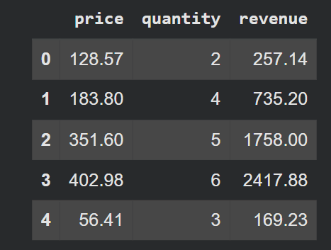
Our goal: compute the total revenue for each order.
df['revenue'] = df['price'] * df['quantity']
display(df[['price', 'quantity', 'revenue']].head())
Output:
# 2. Using a Function for Conditional Logic
When your transformation requires logic that can’t be expressed through simple arithmetic, .apply() allows you to pass a function across a column or row.
Our goal: assign a shipping priority label based on the number of days to ship.
def shipping_label(days):
    if days <= 2:
        return 'Express'
    elif days <= 5:
        return 'Standard'
    else:
        return 'Economy'

df['shipping_tier'] = df['days_to_ship'].apply(shipping_label)
display(df[['days_to_ship', 'shipping_tier']].head())
Output:
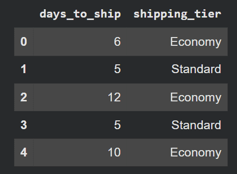
Using .apply() is clean, readable, and much easier to debug than a loop. It’s ideal when your logic is conditional and np.where() or np.select() would feel overly nested.
# 3. Using np.where() for Binary Conditions
When you’re dealing with a binary condition — one result if true, another if false — np.where() is the clean, efficient choice.
Our goal: flag orders where the customer is eligible for a senior discount.
df['senior_discount'] = np.where(df['customer_age'] >= 60, True, False)
display(df[['customer_age', 'senior_discount']].head())
Output:
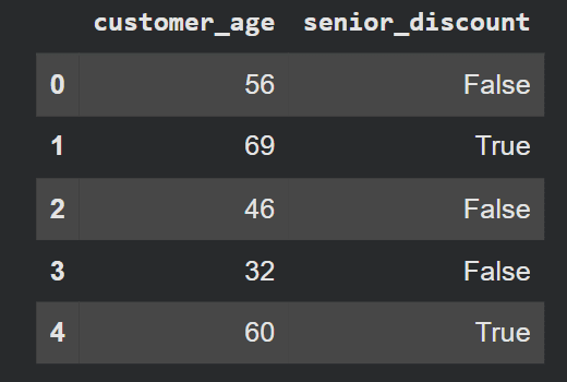
np.where() is fully vectorized and significantly faster than .apply() for straightforward true/false conditions. Think of it as a vectorized ternary operator.
# 4. Handling Multiple Conditions with np.select()
When you have more than two conditions to evaluate, np.select() lets you define a list of conditions and their corresponding values without resorting to nested if/elif chains.
Our goal: assign a region-based tax rate.
conditions = [
    df['region'] == 'North',
    df['region'] == 'South',
    df['region'] == 'East',
    df['region'] == 'West',
]
tax_rates = [0.08, 0.06, 0.07, 0.09]

df['tax_rate'] = np.select(conditions, tax_rates, default=0.07)
df['tax_amount'] = df['price'] * df['tax_rate']
display(df[['region', 'price', 'tax_rate', 'tax_amount']].head())
Output:
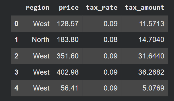
np.select() evaluates all conditions sequentially and picks the first match. The default parameter handles anything that doesn’t match, serving as a useful safety net.
# 5. Mapping Values with a Dictionary Lookup
When you need to translate values in a column — such as mapping category names to numeric codes, or replacing keys with labels — .map() paired with a dictionary is clean and fast.
Our goal: map product categories to internal department codes.
category_codes = {
    'Electronics': 'ELEC',
    'Clothing': 'CLTH',
    'Home & Kitchen': 'HOME',
    'Sports': 'SPRT',
    'Books': 'BOOK',
}

df['dept_code'] = df['product_category'].map(category_codes)
display(df[['product_category', 'dept_code']].head())
Output:
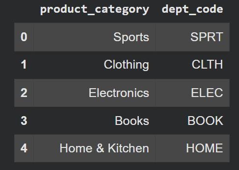
.map() acts like a lookup table. It’s one of the most overlooked tools in pandas — we often default to .apply(lambda x: dict[x]) when .map(dict) accomplishes the same task more quickly.
# 6. Handling Strings with the .str Accessor
String handling is where people most frequently fall back on loops or .apply(). The .str accessor lets you perform string operations across an entire column without either.
Our goal: pull the first word from the product_category column and convert it to lowercase.
df['category_slug'] = df['product_category'].str.split().str[0].str.lower()
display(df[['product_category', 'category_slug']].head())
Output:
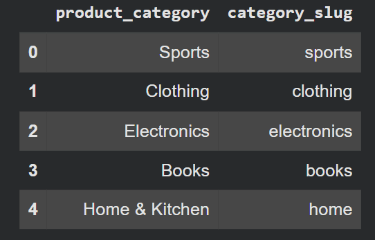
You can chain .str methods just like regular Python string methods. It also supports .str.contains(), .str.replace(), .str.extract() for regex, and more.
# 7. Summarizing Groups with .groupby()
A frequent loop pattern is cycling through subsets of data to compute group-level statistics. .groupby() handles this natively.
Our goal: calculate total revenue and average days to ship per product category.
summary = (
    df.groupby('product_category')
    .agg(
        total_revenue=('revenue', 'sum'),
        avg_ship_days=('days_to_ship', 'mean'),
        order_count=('order_id', 'count')
    )
    .round(2)
    .reset_index()
)
summary
Output:
![]()
# Picking the Right Tool
Most transformations you’d write a loop for fit neatly into one of these patterns:
| Operation / Method | Use Case / Description |
|---|---|
| Arithmetic on columns | Carry out vectorized math operations like addition, subtraction, multiplication, and division directly on DataFrame columns. |
Vectorized operations (*, +, etc.) | Apply element-wise operations across entire columns efficiently without writing explicit loops. |
| Simple true/false condition | Evaluate boolean conditions to filter rows or create conditional columns. |
np.where() | Apply conditional (if-else) logic in a vectorized way for arrays and DataFrame columns. |
| Multiple conditions, multiple outcomes | Handle complex conditional logic with multiple rules and corresponding outputs. |
np.select() | Choose values based on multiple conditions and return the matching outputs. |
| Value substitution via lookup | Swap values using mapping dictionaries for quick transformations. |
.map(dict) | Map values in a Series using a dictionary or function for substitution. |
.apply() | Apply custom functions row-wise or column-wise for flexible transformations. |
| String manipulation |
Use vectorized string operations via the .str accessor for cleaning and transforming text data. |
.groupby() + .agg() | Group data and compute aggregated statistics like sum, mean, count, etc. |
Once you start thinking in terms of columns instead of rows, you’ll find the pandas API starts to feel less like a workaround and more like the way it was designed to be used.
Bala Priya C is a developer and technical writer from India. She enjoys working at the intersection of math, programming, data science, and content creation. Her areas of interest and expertise include DevOps, data science, and natural language processing. She loves reading, writing, coding, and coffee! Currently, she’s focused on learning and sharing her knowledge with the developer community by authoring tutorials, how-to guides, opinion pieces, and more. Bala also creates engaging resource overviews and coding tutorials.