




# Introduction
There’s a satisfying feeling that comes from watching your machine learning model’s loss drop steadily during training—until suddenly, your validation accuracy stalls or the loss shoots up, and you have no idea why. When this happens, most people throw more logging into the mix or start fiddling with hyperparameters, crossing their fingers that something improves. What many practitioners overlook at this stage is getting genuine insight into the internal mechanics of the model as it trains. Visual debugging tools are incredibly valuable at exactly this moment.
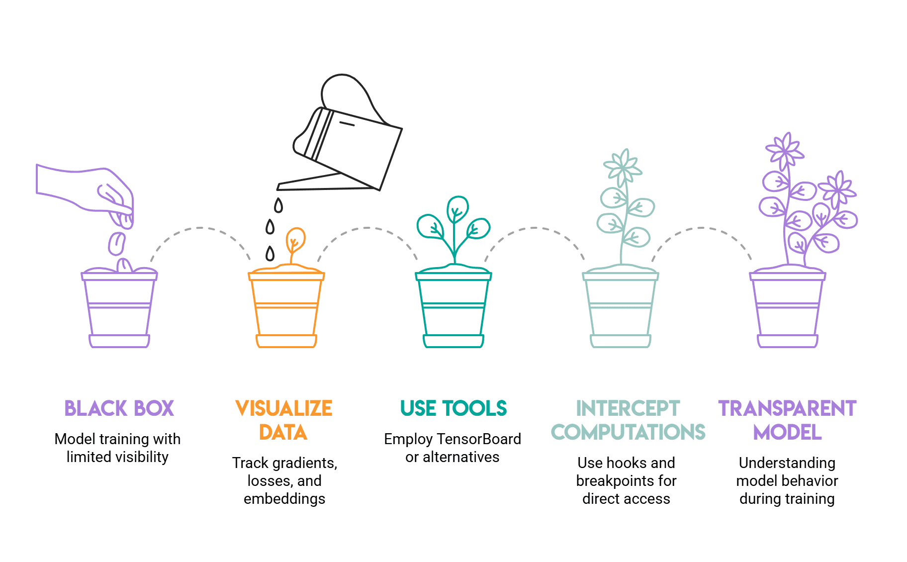
This article explores three key areas: what specific aspects of training to visualize—namely gradients, losses, and embeddings—the tools available for generating those visualizations (TensorBoard and several strong alternatives), and techniques for tapping directly into model computations using hooks and breakpoints.
# Visualizing Gradients, Losses, and Embeddings
// Loss Curves
The loss curve is typically the first plot you reach for while training a model. When both training and validation loss steadily decrease and track closely together, that’s a good sign—training is going smoothly. But when validation loss starts climbing while training loss remains on its way down, the model is overfitting. When both curves flatten out too quickly, the model has stopped learning, which often points to issues with the data or your learning rate.
Beyond that, it’s also important to pay attention to how gradients flow. In practice, a sign of the vanishing gradient problem is loss curves that decrease in a smooth but sluggish manner, suggesting that gradients have become too small by the time they reach the network’s earliest layers.
The plot below illustrates a typical overfitting scenario. For the first ten epochs, both losses drop in tandem, but then the validation loss begins creeping upward while the training loss continues its descent.
The red dotted line marks where the two curves start to diverge: during an actual training run, that’s precisely the moment to start considering regularization or early stopping.
import torch
import torch.nn as nn
import matplotlib.pyplot as plt

model = nn.Sequential(nn.Linear(16, 16), nn.Tanh(),
                      nn.Linear(16, 16), nn.Tanh(),
                      nn.Linear(16, 1))

grad_magnitudes = {}

def grad_hook(name):
    def hook(module, grad_input, grad_output):
        grad_magnitudes[name] = grad_output[0].abs().mean().item()
    return hook

for i, layer in enumerate(model):
    layer.register_backward_hook(grad_hook("Layer {i}"))

output = model(torch.randn(32, 16))
output.mean().backward()

plt.bar(grad_magnitudes.keys(), grad_magnitudes.values())
plt.title("Mean Gradient Magnitude per Layer")
plt.ylabel("Mean |gradient|")
plt.xticks(rotation=15)
plt.tight_layout()
plt.show()
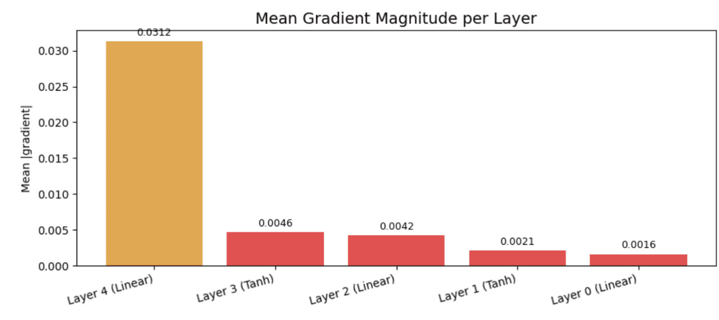
The generated output:
// Raw Gradient Magnitudes
Layer 4 (Linear): 0.031250
Layer 3 (Tanh): 0.004646
Layer 2 (Linear): 0.004241
Layer 1 (Tanh): 0.002126
Layer 0 (Linear): 0.001631
The chart reads from right to left: Layer 4 is the output layer, and Layer 0 is the very first layer. The output layer receives a gradient of about 0.031, but by the time it reaches Layer 0, that value has shrunk to 0.0016—roughly a 20-fold decrease.
The red bar displayed for each of the earliest three layers signals that gradients are already in the danger zone long before they arrive at the network’s input. During an actual training run on a deeper architecture, these initial layers would update their weights at such a slow pace that they would barely learn a thing.
This is a concrete, hands-on demonstration of the vanishing gradient issue: the earliest layers are quietly falling behind, and without a visualization like this, you’d never see it happening.
// Gradient Visualization
Charting gradient magnitudes across each layer during training offers a straightforward way to check if gradients are reaching the network’s earlier layers with meaningful values. In deep architectures, gradients can fade away as they propagate backward through successive layers. Creating histograms of gradient values per layer throughout training can surface this pattern and let you catch the problem early.
In PyTorch, the register_backward_hook lets you capture gradient tensors from any layer without having to alter the training loop. You attach a hook to a module, and it fires on every backward pass, passing gradient tensors to whatever callback you define.
The display below depicts the full spread of gradient values for each layer after a single backward pass. Each subplot corresponds to a single layer, arranged from the network’s first to its last.
The code is available here.
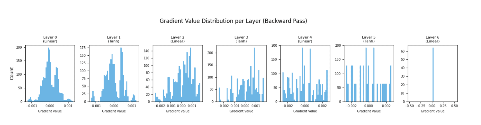
In a well-functioning network, you want to see histograms across all layers that have roughly comparable spreads.
If the earliest layers show a very narrow, spike-like distribution tightly clustered around zero, that’s a warning sign of vanishing gradients.
The gradients technically still exist, but their values are so tiny they carry almost no useful learning signal. Catching this pattern after just a few batches—rather than after completing an entire training run—can save significant time.
// Embeddings
Once a model maps inputs into a learned representation, examining that representation reveals whether the model is differentiating the data as intended. The typical workflow is to extract embeddings from a trained (or partially trained) model, bring their dimensionality down using t-SNE or UMAP, and then plot them with class labels represented as colors.
Well-defined, distinct clusters mean the model has picked up on meaningful separations. Overlapping classes suggest the model hasn’t yet teased apart those concepts. This kind of inspection is particularly helpful for debugging image or text models before attaching the final classification layer.
# TensorBoard and Its Alternatives
// TensorBoard
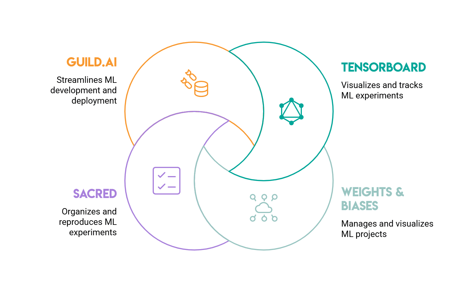
TensorBoard remains the go-to starting point. Originally developed for TensorFlow, it integrates with PyTorch through torch.utils.tensorboard. Logging data is done via a SummaryWriter object, and results are viewable directly in a browser tab. It manages
You can track basic metrics (loss, accuracy), weight and gradient distributions, images, and use an embedding projector to visualize high-dimensional data.
One key limitation is its local focus. To share results with a team, you need to set up shared storage for log files or use TensorBoard.dev, which has certain restrictions on supported features.
// Weights & Biases
Weights & Biases (W&B) is the go-to tool for most machine learning teams who need collaboration features or more in-depth experiment tracking.
Getting started takes just two lines of code: wandb.init() at the beginning of a run and wandb.log() within the training loop. All data automatically syncs to a cloud-based dashboard, and runs are organized by project, making it easy to compare different experiments.
Take a look at the code example below:
import wandb

wandb.init(project="my-model", config={"lr": 0.001, "epochs": 20, "batch_size": 32})

for epoch in range(wandb.config.epochs):
    train_loss = 1 / (1 + 0.3 * epoch)   # simulated
    val_loss   = train_loss + max(0, 0.04 * (epoch - 10))  # simulated
    wandb.log({"epoch": epoch, "train_loss": train_loss, "val_loss": val_loss})

wandb.finish()
After the run completes, all logged metrics appear in the W&B dashboard alongside the configuration that generated them. You can compare two runs with different parameters simply by selecting them in the interface—no need to manually parse log files.
W&B also includes built-in hyperparameter sweep support with visualizations that highlight which parameters had the greatest impact on results.
System-level metrics such as GPU utilization and memory consumption are captured automatically as well. For teams managing many concurrent experiments, the shared workspace significantly reduces the manual effort of keeping track of what’s been tested.
// Sacred
Sacred approaches things differently. Its primary focus is on reproducibility rather than visualization. By annotating a training script with Sacred’s experiment decorator, the entire configuration, any runtime modifications, and all recorded metrics are saved in a database (typically MongoDB). This means every run and its exact settings become a permanent, searchable record.
For visualization, Sacred works alongside front-end tools like Omniboard or Sacredboard. This adds some extra setup complexity compared to TensorBoard or W&B, but the payoff is strong auditability: any past run can be reproduced precisely with its original settings.
// Guild.ai
Guild.ai operates from the command line and doesn’t require any changes to your training code. You execute a training script through Guild with guild run train.py, which captures all script logs and output files, associating them with that specific run. Metrics and run comparisons can be accessed through Guild’s command-line interface (CLI) or its local web UI.
This tool is particularly useful when working with existing scripts or third-party code that you’d rather not alter. It offers fewer features than W&B, but the setup effort is correspondingly minimal.
# Using Breakpoints and Hooks for Machine Learning Computations
// Forward and Backward Hooks
PyTorch’s hook system allows you to intercept computations at any stage of a model’s forward or backward pass. The register_forward_hook function attaches a callback to any layer, triggering each time that layer processes a batch. The callback receives the layer’s input and output tensors, which you can log, check for NaN values, or visualize.
The register_backward_hook function performs the same role during the backward pass, giving you access to gradient tensors flowing through each layer. Between these two hooks, you can inspect nearly anything you’d want during training changes to the model definition or training loop.
A common use case is detecting numerical instability. A forward hook that checks tensor.isnan().any() on every layer’s output catches NaN values immediately, preventing them from propagating further and disrupting the rest of the training.
Here’s a minimal working example using a three-layer model with a hook on each layer:
import torch
import torch.nn as nn

model = nn.Sequential(nn.Linear(8, 16), nn.ReLU(), nn.Linear(16, 4))

def nan_hook(layer, input, output):
    if output.isnan().any():
        print(f"[NaN detected] Layer: {layer.__class__.__name__}")
    else:
        print(f"[Clean] Layer: {layer.__class__.__name__}, output shape: {tuple(output.shape)}")

for layer in model:
    layer.register_forward_hook(nan_hook)

print("--- Normal input ---")
model(torch.randn(2, 8))

print("n--- Corrupted input ---")
bad_input = torch.randn(2, 8)
bad_input[0, 3] = float('nan')
model(bad_input)
Here’s the expected output when executed:
--- Normal input ---

[Clean] Layer: Linear, output shape: (2, 16)
[Clean] Layer: ReLU, output shape: (2, 16)
[Clean] Layer: Linear, output shape: (2, 4)

--- Corrupted input ---

[NaN detected] Layer: Linear
[NaN detected] Layer: ReLU
[NaN detected] Layer: Linear
In this example, the hook examines each layer’s output tensor and reports whether it’s clean or contains corrupted values.
Running it twice—once with normal input and once with a single NaN value injected—shows how numerical instability spreads through the network from layer to layer.
// Debugger Breakpoints
Standard Python debuggers work seamlessly inside training loops.
Inserting import pdb; pdb.set_trace() at any point pauses execution and opens an interactive prompt where you can inspect tensor shapes, verify that data preprocessing isn’t producing unexpected values, and manually step through the forward pass.
Most machine learning development environments—both VSCode and PyCharm—support graphical breakpoints and tensor inspection in a dedicated panel, providing a faster alternative to the terminal-based pdb interface.
Breakpoints are especially useful during the first one or two batches, letting you confirm that the data pipeline, model, and loss function are all behaving correctly before launching a full training run.
# Conclusion
Training a model without visualizing its internal behavior means you’re interpreting symptoms instead of identifying root causes.
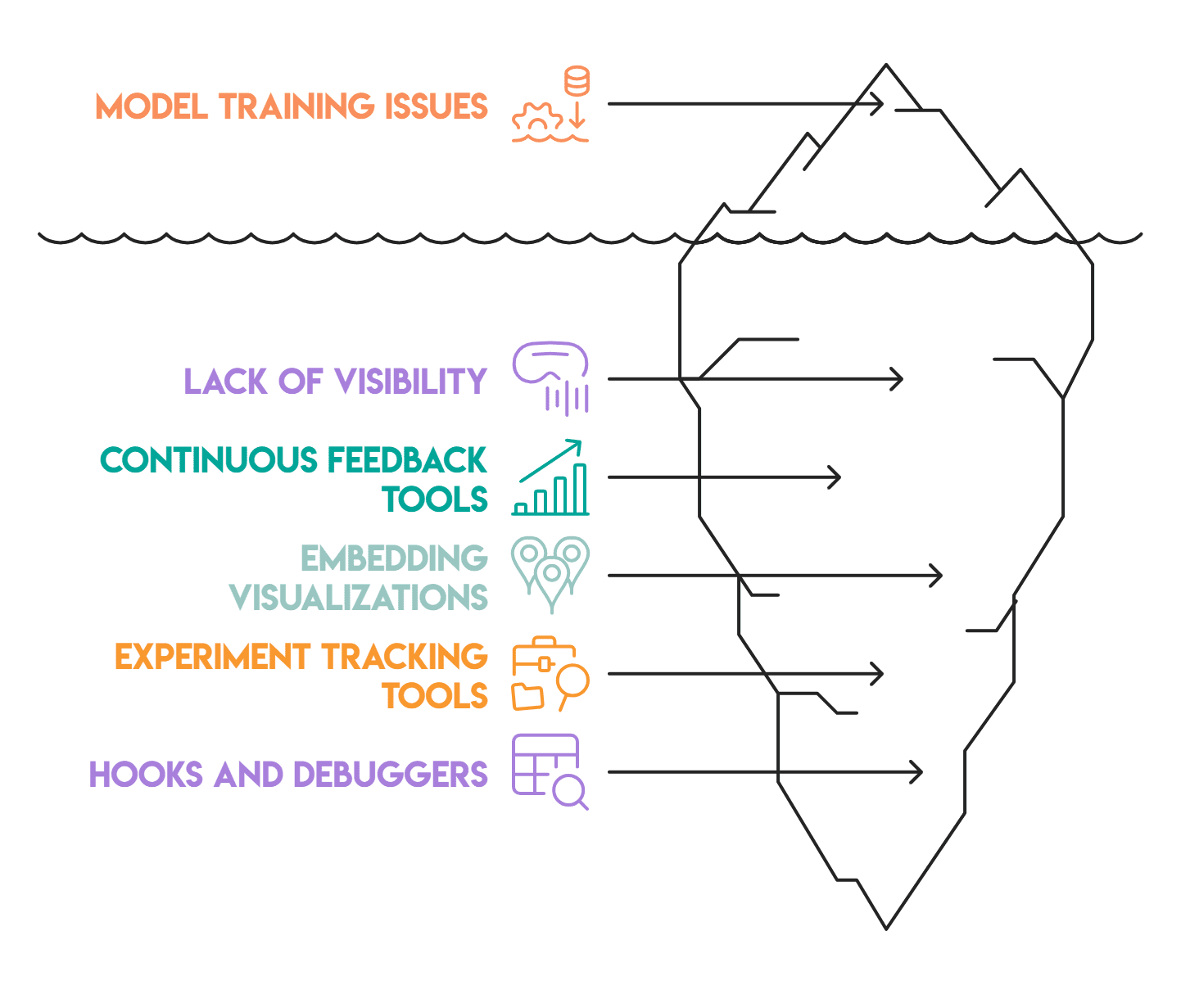
When training a model—whether the loss curve plateaus prematurely, gradients vanish, or embeddings fail to separate—without proper instrumentation, none of these issues will make themselves obvious.
The tools discussed in this article work at multiple levels. Loss curves and gradient histograms provide continuous feedback during training, catching problems like overfitting or vanishing gradients before they compound and derail your project.
Embedding visualizations show whether the model is learning meaningful data separations. TensorBoard, W&B, Sacred, and Guild.ai each handle logging and tracking differently, but they all share the same goal: making experiment history searchable and comparable instead of scattered across files. Finally, hooks and debuggers take things a step further by letting you pause and inspect the actual tensors moving through the network at any layer.
That said, these tools can’t automatically fix a broken model. What they do is reduce the gap between something going wrong and figuring out why—and that’s usually the hardest part of the process.
Nate Rosidi is a data scientist focused on product strategy. He’s also an adjunct professor teaching analytics, and is the founder of StrataScratch, a platform that helps data scientists prepare for interviews with real questions from top companies. Nate writes about the latest career trends, shares interview tips, highlights data science projects, and covers all things SQL.
