


# Introduction
Ever typed a search query and gotten back results that matched your words but missed your point entirely? Or noticed a recommendation engine suggest something surprisingly relevant even though you never explicitly looked for it? The difference between “matching exact words” and “grasping what you actually mean” is what separates a basic search tool from a truly powerful one.
Vector search bridges this gap by turning text into points within a high-dimensional space, where geometric closeness reflects semantic similarity. Two sentences can have zero words in common yet still sit right next to each other — because the model has learned that their meanings are alike.
This guide walks you through building a vector search engine entirely from scratch in Python using nothing but NumPy, so you can understand precisely what happens at every stage: how embeddings are stored and normalized, why cosine similarity simplifies into a dot product, and what the search space actually looks like when projected down to two dimensions.
You can find the full code on GitHub.
# What Is Vector Search?
Conventional keyword search hunts for exact word matches. Vector search takes a different approach: it transforms both documents and queries into numerical vectors known as embeddings, then identifies which vectors are nearest to each other in a high-dimensional space.
The core idea is that proximity in vector space equals semantic similarity. Two sentences conveying the same meaning — even with no shared vocabulary — will produce embeddings positioned close together.
The distance metric you choose to define “nearness” is what powers the entire system. The most widely used option is cosine similarity, which measures the angle between two vectors rather than their absolute distance. This property makes it scale-invariant — ideal when you care about direction or meaning rather than magnitude or word count.
# Setting Up the Dataset
We’ll use a collection of brief product descriptions from a fictional online store. These are pre-embedded as 8-dimensional vectors — a significantly reduced dimensionality that’s still realistic enough to illustrate the key concepts.
In a production system, you’d generate these embeddings using a model like sentence-transformers. For this walkthrough, we simulate that step using controlled random data with a well-defined cluster structure.
import numpy as np

np.random.seed(42)

# Product catalog — 3 semantic clusters: electronics, clothing, furniture
products = [
    "Wireless noise-cancelling headphones with 30-hour battery",
    "Bluetooth speaker with waterproof design",
    "USB-C hub with 7 ports and power delivery",
    "4K HDMI cable 6ft braided",
    "Mechanical keyboard with RGB backlight",
    "Men's slim-fit chino pants navy blue",
    "Women's merino wool turtleneck sweater",
    "Unisex running jacket lightweight windbreaker",
    "Leather chelsea boots for men",
    "Organic cotton crew neck t-shirt",
    "Solid oak dining table seats 6",
    "Ergonomic mesh office chair lumbar support",
    "Linen sofa 3-seater natural beige",
    "Bamboo bookshelf 5-tier adjustable",
    "Memory foam mattress queen size medium firm",
]

# Simulate embeddings with cluster structure
# Cluster centers in 8D space
electronics_center = np.array([0.9, 0.1, 0.2, 0.8, 0.1, 0.3, 0.7, 0.2])
clothing_center    = np.array([0.1, 0.8, 0.7, 0.1, 0.9, 0.2, 0.1, 0.8])
furniture_center   = np.array([0.2, 0.3, 0.9, 0.2, 0.1, 0.9, 0.3, 0.1])

n_per_cluster = 5
noise = 0.08

embeddings = np.vstack([
    electronics_center + np.random.randn(n_per_cluster, 8) * noise,
    clothing_center    + np.random.randn(n_per_cluster, 8) * noise,
    furniture_center   + np.random.randn(n_per_cluster, 8) * noise,
])

print(f"Embeddings shape: {embeddings.shape}")
Output:
Embeddings shape: (15, 8)Each row represents a product. Each column corresponds to one dimension of its embedding. The product names won’t be used by the search engine itself — only the embeddings carry weight.
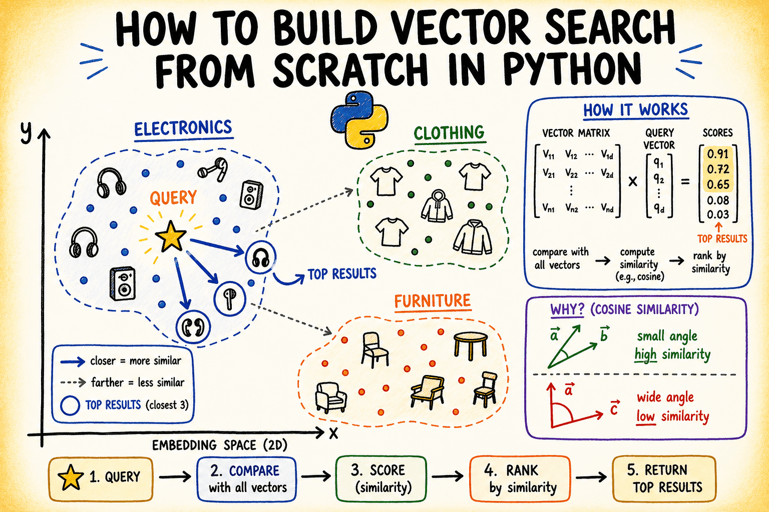
Image by Author
# Building the Index
The “index” in a vector search engine is simply the collection of stored, normalized embeddings. Normalization matters here because it turns cosine similarity into a dot product — a much cheaper operation to compute.
def normalize(vectors: np.ndarray) -> np.ndarray:
    """L2-normalize each row vector."""
    norms = np.linalg.norm(vectors, axis=1, keepdims=True)
    # Avoid division by zero
    norms = np.where(norms == 0, 1e-10, norms)
    return vectors / norms

class VectorIndex:
    def __init__(self):
        self.vectors = None
        self.labels = None

    def add(self, vectors: np.ndarray, labels: list):
        self.vectors = normalize(vectors)
        self.labels = labels
        print(f"Indexed {len(labels)} items with {vectors.shape[1]}-dimensional embeddings.")

    def search(self, query_vector: np.ndarray, top_k: int = 3):
        query_norm = normalize(query_vector.reshape(1, -1))
        # Cosine similarity = dot product of normalized vectors
        scores = self.vectors @ query_norm.T  # shape: (n_items, 1)
        scores = scores.flatten()
        # Get top-k indices sorted by descending score
        top_indices = np.argsort(scores)[::-1][:top_k]
        return [(self.labels[i], float(scores[i])) for i in top_indices]

index = VectorIndex()
index.add(embeddings, products)
Output:
Indexed 15 items with 8-dimensional embeddings.The search method performs three steps: it normalizes the query, computes dot products against every stored vector, then sorts by score and returns the top-k matches. That single matrix multiplication (self.vectors @ query_norm.T) is the entire retrieval process.
# Running Queries
Now let’s put our engine to the test with a few sample queries. We build query vectors by taking one of the cluster centers and adding a small amount of noise to mimic a real-world query embedding.
def make_query(center: np.ndarray, noise_scale: float = 0.05) -> np.ndarray:
    return center + np.random.randn(8) * noise_scale


queries = {
    "audio equipment": make_query(electronics_center),
"casual wear":     make_query(clothing_center),
    "home furniture":  make_query(furniture_center),
}

for query_name, q_vec in queries.items():
    print(f"nQuery: '{query_name}'")
    results = index.search(q_vec, top_k=3)
    for rank, (label, score) in enumerate(results, 1):
        print(f"  {rank}. [{score:.4f}] {label}")
Here’s what the output looks like:
Query: 'audio equipment'
  1. [0.9856] Wireless noise-cancelling headphones with 30-hour battery
  2. [0.9840] USB-C hub with 7 ports and power delivery
  3. [0.9829] Mechanical keyboard with RGB backlight

Query: 'casual wear'
  1. [0.9960] Men's slim-fit chino pants navy blue
  2. [0.9958] Leather chelsea boots for men
  3. [0.9916] Women's merino wool turtleneck sweater

Query: 'home furniture'
  1. [0.9929] Bamboo bookshelf 5-tier adjustable
  2. [0.9902] Linen sofa 3-seater natural beige
  3. [0.9881] Solid oak dining table seats 6
When scores are near 1.0, it means the query and document point in almost the same direction within the embedding space — which is precisely what you’d expect when both are derived from the same cluster center.
# Visualizing the Embedding Space
It’s tough to get an intuitive feel for data living in many dimensions. Principal Component Analysis (PCA) squashes those 8-dimensional embeddings down into 2D, letting you actually see how the clusters are arranged. Below is a stripped-down PCA implementation using nothing but NumPy.
The code below calculates the 2D PCA projection and renders all product embeddings, complete with labels and cluster-specific colors:
import matplotlib.pyplot as plt
import matplotlib.patches as mpatches

projected = pca_2d(embeddings)

cluster_colors = (
    ["#4A90D9"] * 5 +   # electronics — blue
    ["#E8734A"] * 5 +   # clothing — orange
    ["#5BAD72"] * 5     # furniture — green
)
cluster_labels = ["Electronics"] * 5 + ["Clothing"] * 5 + ["Furniture"] * 5

fig, ax = plt.subplots(figsize=(6, 4))
ax.scatter(projected[:, 0], projected[:, 1],
           c=cluster_colors, s=100, edgecolors="white", linewidths=0.7, zorder=3)
Next, the query vectors are projected into the same 2D space, overlaid onto the scatter plot, and the figure is finalized:
# Plot query projections
q_projected = pca_2d(
    np.vstack(list(queries.values())) - embeddings.mean(axis=0)
)
for (qname, _), (qx, qy) in zip(queries.items(), q_projected):
    ax.scatter(qx, qy, marker="*", s=200, color="gold",
               edgecolors="#333", linewidths=0.6, zorder=4)
    ax.annotate(f"⟵ query: {qname}", (qx, qy),
                textcoords="offset points", xytext=(6, -8),
                fontsize=7, color="#555555", style="italic")

legend_patches = [
    mpatches.Patch(color="#4A90D9", label="Electronics"),
    mpatches.Patch(color="#E8734A", label="Clothing"),
    mpatches.Patch(color="#5BAD72", label="Furniture"),
    mpatches.Patch(color="gold",    label="Query vectors"),
]
ax.legend(handles=legend_patches, loc="upper left", fontsize=6)
ax.set_title("Vector Search — Embedding Space (PCA projection)", fontsize=10, pad=10)
ax.set_xlabel("PC 1"); ax.set_ylabel("PC 2")
ax.grid(True, linestyle="--", alpha=0.4)
plt.tight_layout()
plt.savefig("embedding_space_queries_only.png", dpi=150)
plt.show()
Output:
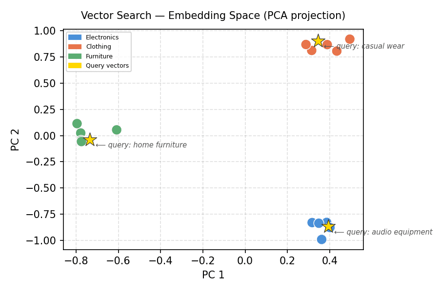
Vector Search — Embedding Space (PCA projection)
The clusters are cleanly separated. Each gold star — representing a query vector — sits right inside the cluster it was built from. This spatial arrangement is exactly what vector search relies on under the hood.
# Visualizing the Similarity Score Distribution
For any given query, it helps to look at how similarity scores spread across the entire index — not just the top-k results. This reveals whether the leading result is a standout match or only slightly better than the rest.
q_vec_furniture = queries["home furniture"]
q_norm_furniture = normalize(q_vec_furniture.reshape(1, -1))
all_scores_furniture = (index.vectors @ q_norm_furniture.T).flatten()

sorted_idx_furniture = np.argsort(all_scores_furniture)[::-1]
sorted_scores_furniture = all_scores_furniture[sorted_idx_furniture]
sorted_labels_furniture = [products[i][:30] + "…" if len(products[i]) > 30
                           else products[i] for i in sorted_idx_furniture]

# Define bar colors: green for furniture items, gray for others
bar_colors_furniture = []
for i in sorted_idx_furniture:
    if i >= 10 and i <= 14:  # Furniture items are originally at indices 10-14
        bar_colors_furniture.append("#5BAD72") # Green for furniture
    else:
        bar_colors_furniture.append("#cccccc") # Gray for others

fig, ax = plt.subplots(figsize=(10, 5))
bars = ax.barh(sorted_labels_furniture[::-1], sorted_scores_furniture[::-1],
               color=bar_colors_furniture[::-1], edgecolor="white", height=0.65)

ax.axvline(sorted_scores_furniture[2], color="#5BAD72", linestyle="--",
           linewidth=1.2, label="Top-3 cutoff")
ax.set_xlim(sorted_scores_furniture.min() - 0.002, 1.001)
ax.set_xlabel("Cosine Similarity Score")
ax.set_title("Query: 'home furniture' — Similarity Across All Products", fontsize=11, pad=12)
ax.legend(fontsize=8)
ax.grid(axis="x", linestyle="--", alpha=0.4)
plt.tight_layout()
plt.savefig("score_distribution_furniture.png", dpi=150)
plt.show()
Output:
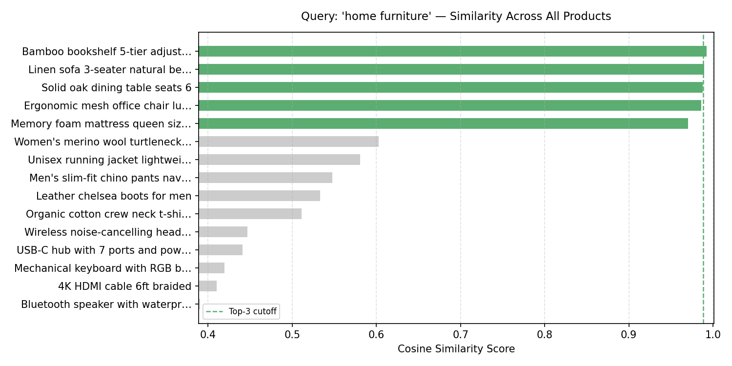
Query: ‘home furniture’ — Similarity Across All Products
There’s a noticeable gap between the furniture cluster (the top 5 bars) and everything else. In a real-world scenario, you could leverage this gap to define a similarity threshold — any results falling below it would be filtered out entirely.
# Wrapping Up
With roughly 50 lines of NumPy, you’ve built a fully functional vector search engine: an index class that normalizes and stores embeddings, a search method leveraging matrix multiplication for cosine similarity, and two visualizations that expose the geometric structure driving the results.
The natural next step is swapping out the simulated embeddings for real ones. Try loading sentence-transformers and embedding your own text corpus — the index code here will work as-is with no modifications needed.
If you enjoy these “built from scratch” walkthroughs, drop a comment and let us know what you’d like to see covered next!
Bala Priya C is a developer and technical writer from India. She loves exploring the crossroads of math, programming, data science, and content creation. Her focus areas include DevOps, data science, and natural language processing. When she’s not reading, writing, coding, or sipping coffee, she’s busy learning and sharing knowledge with the developer community through tutorials, how-to guides, opinion pieces, and more. Bala also puts together resource overviews and coding tutorials.