


At first look, including extra options to a mannequin looks like an apparent method to enhance efficiency. If a mannequin can study from extra data, it ought to be capable of make higher predictions. In observe, nevertheless, this intuition usually introduces hidden structural dangers. Each extra function creates one other dependency on upstream knowledge pipelines, exterior techniques, and knowledge high quality checks. A single lacking subject, schema change, or delayed dataset can quietly degrade predictions in manufacturing.
The deeper subject will not be computational value or system complexity — it’s weight instability. In regression fashions, particularly when options are correlated or weakly informative, the optimizer struggles to assign credit score in a significant method. Coefficients can shift unpredictably because the mannequin makes an attempt to distribute affect throughout overlapping alerts, and low-signal variables might seem essential merely on account of noise within the knowledge. Over time, this results in fashions that look subtle on paper however behave inconsistently when deployed.
On this article, we’ll look at why including extra options could make regression fashions much less dependable moderately than extra correct. We are going to discover how correlated options distort coefficient estimates, how weak alerts get mistaken for actual patterns, and why every extra function will increase manufacturing fragility. To make these concepts concrete, we’ll stroll by examples utilizing a property pricing dataset and evaluate the habits of enormous “kitchen-sink” fashions with leaner, extra secure options.
Importing the dependencies
pip set up seaborn scikit-learn pandas numpy matplotlibimport numpy as np
import pandas as pd
import matplotlib.pyplot as plt
import matplotlib.gridspec as gridspec
import seaborn as sns
from sklearn.linear_model import Ridge
from sklearn.preprocessing import StandardScaler
from sklearn.metrics import mean_squared_error
from sklearn.model_selection import train_test_split
import warnings
warnings.filterwarnings("ignore")
plt.rcParams.replace({
"figure.facecolor": "#FAFAFA",
"axes.facecolor": "#FAFAFA",
"axes.spines.top": False,
"axes.spines.right":False,
"axes.grid": True,
"grid.color": "#E5E5E5",
"grid.linewidth": 0.8,
"font.family": "monospace",
})
SEED = 42
np.random.seed(SEED)
This code units a clear, constant Matplotlib model by adjusting background colours, grid look, and eradicating pointless axis spines for clearer visualizations. It additionally units a hard and fast NumPy random seed (42) to make sure that any randomly generated knowledge stays reproducible throughout runs.
Artificial Property Dataset
N = 800   # coaching samples

# ── True sign options ────────────────────────────────────
sqft          = np.random.regular(1800, 400, N)          # sturdy sign
bedrooms      = np.spherical(sqft / 550 + np.random.regular(0, 0.4, N)).clip(1, 6)
neighborhood  = np.random.alternative([0, 1, 2], N, p=[0.3, 0.5, 0.2])  # categorical

# ── Derived / correlated options (multicollinearity) ───────
total_rooms   = bedrooms + np.random.regular(2, 0.3, N)       # ≈ bedrooms
floor_area_m2 = sqft * 0.0929 + np.random.regular(0, 1, N)   # ≈ sqft in m²
lot_sqft      = sqft * 1.4    + np.random.regular(0, 50, N)   # ≈ sqft scaled

# ── Weak / spurious options ────────────────────────────────
door_color_code  = np.random.randint(0, 10, N).astype(float)
bus_stop_age_yrs = np.random.regular(15, 5, N)
nearest_mcdonalds_m = np.random.regular(800, 200, N)

# ── Pure noise options (simulate 90 random columns) ────────
noise_features = np.random.randn(N, 90)
noise_df = pd.DataFrame(
    noise_features,
    columns=[f"noise_{i:03d}" for i in range(90)]
)

# ── Goal: home worth ─────────────────────────────────────
worth = (
      120 * sqft
    + 8_000 * bedrooms
    + 30_000 * neighborhood
    - 15 * bus_stop_age_yrs          # tiny actual impact
    + np.random.regular(0, 15_000, N) # irreducible noise
)

# ── Assemble DataFrames ──────────────────────────────────────
signal_cols = ["sqft", "bedrooms", "neighborhood",
               "total_rooms", "floor_area_m2", "lot_sqft",
               "door_color_code", "bus_stop_age_yrs",
               "nearest_mcdonalds_m"]

df_base = pd.DataFrame({
    "sqft": sqft,
    "bedrooms": bedrooms,
    "neighborhood": neighborhood,
    "total_rooms": total_rooms,
    "floor_area_m2": floor_area_m2,
    "lot_sqft": lot_sqft,
    "door_color_code": door_color_code,
    "bus_stop_age_yrs": bus_stop_age_yrs,
    "nearest_mcdonalds_m": nearest_mcdonalds_m,
    "price": worth,
})

df_full = pd.concat([df_base.drop("price", axis=1), noise_df,
                     df_base[["price"]]], axis=1)

LEAN_FEATURES  = ["sqft", "bedrooms", "neighborhood"]
NOISY_FEATURES = [c for c in df_full.columns if c != "price"]

print(f"Lean model features : {len(LEAN_FEATURES)}")
print(f"Noisy model features: {len(NOISY_FEATURES)}")
print(f"Dataset shape       : {df_full.shape}")
This code constructs an artificial dataset designed to imitate a real-world property pricing state of affairs, the place solely a small variety of variables really affect the goal whereas many others introduce redundancy or noise. The dataset accommodates 800 coaching samples. Core sign options reminiscent of sq. footage (sqft), variety of bedrooms, and neighborhood class characterize the first drivers of home costs. Along with these, a number of derived options are deliberately created to be extremely correlated with the core variables—reminiscent of floor_area_m2 (a unit conversion of sq. footage), lot_sqft, and total_rooms. These variables simulate multicollinearity, a standard subject in actual datasets the place a number of options carry overlapping data.
The dataset additionally contains weak or spurious options—reminiscent of door_color_code, bus_stop_age_yrs, and nearest_mcdonalds_m—which have little or no significant relationship with property worth. To additional replicate the “kitchen-sink model” drawback, the script generates 90 utterly random noise options, representing irrelevant columns that usually seem in massive datasets. The goal variable worth is constructed utilizing a identified components the place sq. footage, bedrooms, and neighborhood have the strongest affect, whereas bus cease age has a really small impact and random noise introduces pure variability.
Lastly, two function units are outlined: a lean mannequin containing solely the three true sign options (sqft, bedrooms, neighborhood) and a loud mannequin containing each out there column besides the goal. This setup permits us to straight evaluate how a minimal, high-signal function set performs in opposition to a big, feature-heavy mannequin stuffed with redundant and irrelevant variables.
Weight Dilution through Multicollinearity
print("n── Correlation between correlated feature pairs ──")
corr_pairs = [
("sqft", "floor_area_m2"),
("sqft", "lot_sqft"),
("bedrooms", "total_rooms"),
]
for a, b in corr_pairs:
r = np.corrcoef(df_full[a], df_full[b])[0, 1]
print(f" {a:20s} ↔ {b:20s} r = {r:.3f}")
fig, axes = plt.subplots(1, 3, figsize=(14, 4))
fig.suptitle("Weight Dilution: Correlated Feature Pairs",
fontsize=13, fontweight="bold", y=1.02)
for ax, (a, b) in zip(axes, corr_pairs):
ax.scatter(df_full[a], df_full[b],
alpha=0.25, s=12, colour="#3B6FD4")
r = np.corrcoef(df_full[a], df_full[b])[0, 1]
ax.set_title(f"r = {r:.3f}", fontsize=11)
ax.set_xlabel(a); ax.set_ylabel(b)
plt.tight_layout()
plt.savefig("01_multicollinearity.png", dpi=150, bbox_inches="tight")
plt.present()
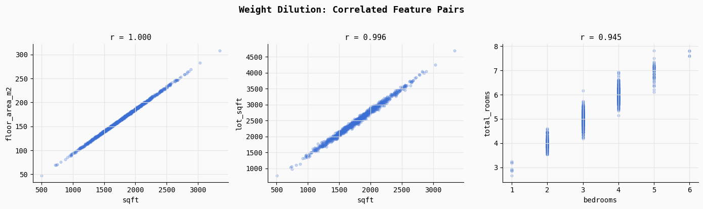
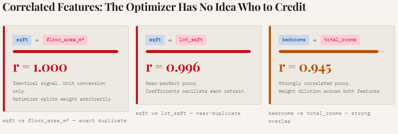
print("Saved → 01_multicollinearity.png")This part demonstrates multicollinearity, a state of affairs the place a number of options include practically equivalent data. The code computes correlation coefficients for 3 deliberately correlated function pairs: sqft vs floor_area_m2, sqft vs lot_sqft, and bedrooms vs total_rooms.

Because the printed outcomes present, these relationships are extraordinarily sturdy (r ≈ 1.0, 0.996, and 0.945), which means the mannequin receives a number of alerts describing the identical underlying property attribute.
The scatter plots visualize this overlap. As a result of these options transfer nearly completely collectively, the regression optimizer struggles to find out which function ought to obtain credit score for predicting the goal. As an alternative of assigning a transparent weight to 1 variable, the mannequin usually splits the affect throughout correlated options in arbitrary methods, resulting in unstable and diluted coefficients. This is likely one of the key explanation why including redundant options could make a mannequin much less interpretable and fewer secure, even when predictive efficiency initially seems comparable.
Weight Instability Throughout Retraining Cycles
N_CYCLES = 30
SAMPLE_SZ = 300 # measurement of every retraining slice
scaler_lean = StandardScaler()
scaler_noisy = StandardScaler()
# Match scalers on full knowledge so items are comparable
X_lean_all = scaler_lean.fit_transform(df_full[LEAN_FEATURES])
X_noisy_all = scaler_noisy.fit_transform(df_full[NOISY_FEATURES])
y_all = df_full["price"].values
lean_weights = [] # form: (N_CYCLES, 3)
noisy_weights = [] # form: (N_CYCLES, 3) -- first 3 cols just for comparability
for cycle in vary(N_CYCLES):
idx = np.random.alternative(N, SAMPLE_SZ, change=False)
X_l = X_lean_all[idx]; y_c = y_all[idx]
X_n = X_noisy_all[idx]
m_lean = Ridge(alpha=1.0).match(X_l, y_c)
m_noisy = Ridge(alpha=1.0).match(X_n, y_c)
lean_weights.append(m_lean.coef_)
noisy_weights.append(m_noisy.coef_[:3]) # sqft, bedrooms, neighborhood
lean_weights = np.array(lean_weights)
noisy_weights = np.array(noisy_weights)
print("n── Coefficient Std Dev across 30 retraining cycles ──")
print(f"{'Feature':<18} {'Lean σ':>10} {'Noisy σ':>10} {'Amplification':>14}")
for i, feat in enumerate(LEAN_FEATURES):
sl = lean_weights[:, i].std()
sn = noisy_weights[:, i].std()
print(f" {feat:<16} {sl:>10.1f} {sn:>10.1f} ×{sn/sl:.1f}")
fig, axes = plt.subplots(1, 3, figsize=(15, 4))
fig.suptitle("Weight Instability: Lean vs. Noisy Model (30 Retraining Cycles)",
fontsize=13, fontweight="bold", y=1.02)
colours = {"lean": "#2DAA6E", "noisy": "#E05C3A"}
for i, feat in enumerate(LEAN_FEATURES):
ax = axes[i]
ax.plot(lean_weights[:, i], colour=colours["lean"],
linewidth=2, label="Lean (3 features)", alpha=0.9)
ax.plot(noisy_weights[:, i], colour=colours["noisy"],
linewidth=2, label="Noisy (100+ features)", alpha=0.9, linestyle="--")
ax.set_title(f'Coefficient: "{feat}"', fontsize=11)
ax.set_xlabel("Retraining Cycle")
ax.set_ylabel("Standardised Weight")
if i == 0:
ax.legend(fontsize=9)
plt.tight_layout()
plt.savefig("02_weight_instability.png", dpi=150, bbox_inches="tight")
plt.present()
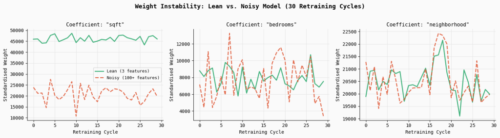
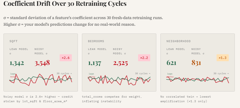
print("Saved → 02_weight_instability.png")This experiment simulates what occurs in actual manufacturing techniques the place fashions are periodically retrained on recent knowledge. Over 30 retraining cycles, the code randomly samples subsets of the dataset and matches two fashions: a lean mannequin utilizing solely the three core sign options, and a loud mannequin utilizing the total function set containing correlated and random variables. By monitoring the coefficients of the important thing options throughout every retraining cycle, we will observe how secure the discovered weights stay over time.
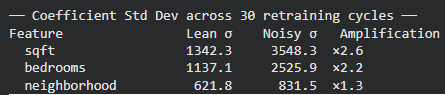
The outcomes present a transparent sample: the noisy mannequin reveals considerably larger coefficient variability.
For instance, the usual deviation of the sqft coefficient will increase by 2.6×, whereas bedrooms turns into 2.2× extra unstable in comparison with the lean mannequin. The plotted strains make this impact visually apparent—the lean mannequin’s coefficients stay comparatively clean and constant throughout retraining cycles, whereas the noisy mannequin’s weights fluctuate way more. This instability arises as a result of correlated and irrelevant options power the optimizer to redistribute credit score unpredictably, making the mannequin’s habits much less dependable even when general accuracy seems comparable.
Sign-to-Noise Ratio (SNR) Degradation
correlations = df_full[NOISY_FEATURES + ["price"]].corr()["price"].drop("price")
correlations = correlations.abs().sort_values(ascending=False)
fig, ax = plt.subplots(figsize=(14, 5))
bar_colors = [
"#2DAA6E" if f in LEAN_FEATURES
else "#E8A838" if f in ["total_rooms", "floor_area_m2", "lot_sqft",
"bus_stop_age_yrs"]
else "#CCCCCC"
for f in correlations.index
]
ax.bar(vary(len(correlations)), correlations.values,
colour=bar_colors, width=0.85, edgecolor="none")
# Legend patches
from matplotlib.patches import Patch
legend_elements = [
Patch(facecolor="#2DAA6E", label="High-signal (lean set)"),
Patch(facecolor="#E8A838", label="Correlated / low-signal"),
Patch(facecolor="#CCCCCC", label="Pure noise"),
]
ax.legend(handles=legend_elements, fontsize=10, loc="upper right")
ax.set_title("Signal-to-Noise Ratio: |Correlation with Price| per Feature",
fontsize=13, fontweight="bold")
ax.set_xlabel("Feature rank (sorted by |r|)")
ax.set_ylabel("|Pearson r| with price")
ax.set_xticks([])
plt.tight_layout()
plt.savefig("03_snr_degradation.png", dpi=150, bbox_inches="tight")
plt.present()
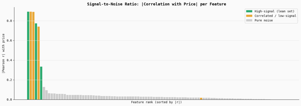
print("Saved → 03_snr_degradation.png")This part measures the sign energy of every function by computing its absolute correlation with the goal variable (worth). The bar chart ranks all options by their correlation, highlighting the true high-signal options in inexperienced, correlated or weak options in orange, and the big set of pure noise options in grey.
The visualization exhibits that solely a small variety of variables carry significant predictive sign, whereas the bulk contribute little to none. When many low-signal or noisy options are included in a mannequin, they dilute the general signal-to-noise ratio, making it more durable for the optimizer to persistently establish the options that really matter.
Characteristic Drift Simulation
def predict_with_drift(mannequin, scaler, X_base, drift_col_idx,
drift_magnitude, feature_cols):
"""Inject drift into one feature column and measure prediction shift."""
X_drifted = X_base.copy()
X_drifted[:, drift_col_idx] += drift_magnitude
return mannequin.predict(scaler.remodel(X_drifted))
# Re-fit each fashions on the total dataset
sc_lean = StandardScaler().match(df_full[LEAN_FEATURES])
sc_noisy = StandardScaler().match(df_full[NOISY_FEATURES])
m_lean_full = Ridge(alpha=1.0).match(
sc_lean.remodel(df_full[LEAN_FEATURES]), y_all)
m_noisy_full = Ridge(alpha=1.0).match(
sc_noisy.remodel(df_full[NOISY_FEATURES]), y_all)
X_lean_raw = df_full[LEAN_FEATURES].values
X_noisy_raw = df_full[NOISY_FEATURES].values
base_lean = m_lean_full.predict(sc_lean.remodel(X_lean_raw))
base_noisy = m_noisy_full.predict(sc_noisy.remodel(X_noisy_raw))
# Drift the "bus_stop_age_yrs" function (low-signal, but in noisy mannequin)
drift_col_noisy = NOISY_FEATURES.index("bus_stop_age_yrs")
drift_range = np.linspace(0, 20, 40) # as much as 20-year drift in bus cease age
rmse_lean_drift, rmse_noisy_drift = [], []
for d in drift_range:
preds_noisy = predict_with_drift(
m_noisy_full, sc_noisy, X_noisy_raw,
drift_col_noisy, d, NOISY_FEATURES)
# Lean mannequin would not even have this function → unaffected
rmse_lean_drift.append(
np.sqrt(mean_squared_error(base_lean, base_lean))) # 0 by design
rmse_noisy_drift.append(
np.sqrt(mean_squared_error(base_noisy, preds_noisy)))
fig, ax = plt.subplots(figsize=(10, 5))
ax.plot(drift_range, rmse_lean_drift, colour="#2DAA6E",
linewidth=2.5, label="Lean model (feature not present)")
ax.plot(drift_range, rmse_noisy_drift, colour="#E05C3A",
linewidth=2.5, linestyle="--",
label="Noisy mannequin ("bus_stop_age_yrs" drifts)")
ax.fill_between(drift_range, rmse_noisy_drift,
alpha=0.15, colour="#E05C3A")
ax.set_xlabel("Feature Drift Magnitude (years)", fontsize=11)
ax.set_ylabel("Prediction Shift RMSE ($)", fontsize=11)
ax.set_title("Feature Drift Sensitivity:nEach Extra Feature = Extra Failure Point",
fontsize=13, fontweight="bold")
ax.legend(fontsize=10)
plt.tight_layout()
plt.savefig("05_drift_sensitivity.png", dpi=150, bbox_inches="tight")
plt.present()
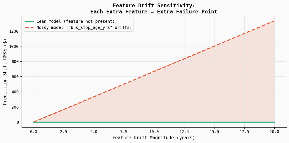
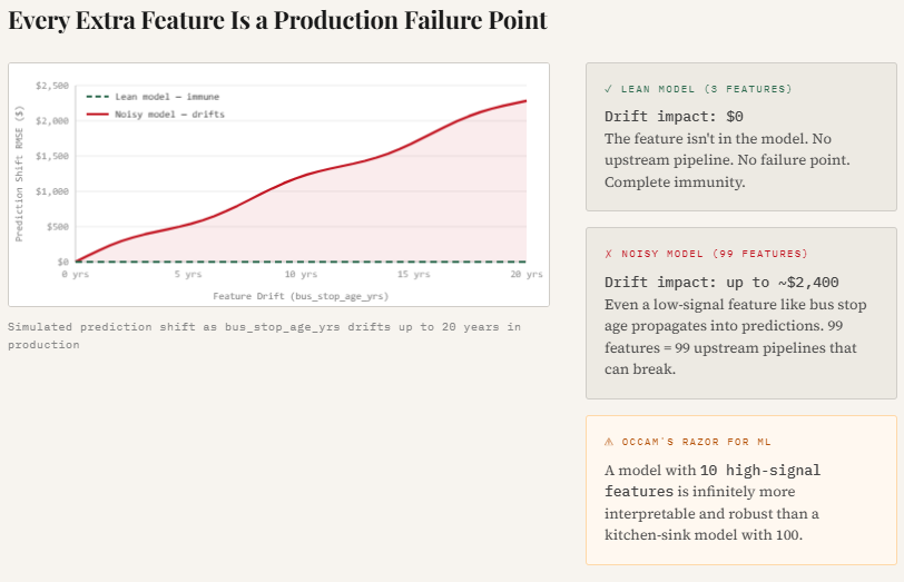
print("Saved → 05_drift_sensitivity.png")This experiment illustrates how function drift can silently have an effect on mannequin predictions in manufacturing. The code introduces gradual drift right into a weak function (bus_stop_age_yrs) and measures how a lot the mannequin’s predictions change. Because the lean mannequin doesn’t embrace this function, its predictions stay utterly secure, whereas the noisy mannequin turns into more and more delicate because the drift magnitude grows.
The ensuing plot exhibits prediction error steadily rising because the function drifts, highlighting an essential manufacturing actuality: each extra function turns into one other potential failure level. Even low-signal variables can introduce instability if their knowledge distribution shifts or upstream pipelines change.
Take a look at the Full Codes right here. Additionally, be at liberty to observe us on Twitter and don’t overlook to affix our 120k+ ML SubReddit and Subscribe to our Publication. Wait! are you on telegram? now you possibly can be part of us on telegram as effectively.

I’m a Civil Engineering Graduate (2022) from Jamia Millia Islamia, New Delhi, and I’ve a eager curiosity in Information Science, particularly Neural Networks and their utility in varied areas.