


# Adjusting Language Models on Apple Silicon Using MLX
Adjusting a language model to your needs once meant paying for cloud GPU time and watching costs climb. If you have a Mac running an Apple Silicon chip, you can now tailor an open model to your own information right on your device, with no cloud expenses and without any of your data leaving your machine.
My journey away from Windows and Dell computers to Mac began in 2014, and I haven’t regretted it since. What began as interest in a neater operating system grew into a genuine admiration for how seamlessly Apple combines hardware with software. More than ten years later, that tight combination is delivering benefits I never expected, most notably the ability to adjust language models directly on the device, cloud charges and with complete data privacy.
This on-device capability is made possible by MLX, an open-source array framework developed by Apple’s machine learning research group, along with its companion toolkit MLX LM, which enables text generation and fine-tuning across countless open models through just a handful of commands. This guide takes you through the entire workflow from start to finish: setting up the tools, structuring a dataset, training a LoRA adapter, reducing memory consumption through quantization, and finally evaluating and deploying the result. By the time you finish, you’ll have a personalized model operating on your own hardware and a repeatable process you can apply to any dataset.
# Why MLX Works So Well on Apple Silicon
Most local inference solutions were originally built for NVIDIA hardware and later adapted for Mac. MLX took a completely different approach. Apple’s research team created it from the ground up to leverage the unified memory design of Apple Silicon, where the CPU and GPU draw from one shared memory pool.
This design eliminates the data-copying step that normally shuttles information back and forth between system RAM and dedicated GPU memory. On a 16 GB Mac, the model parameters, optimizer states, and training batch all live within the same memory space, making on-device fine-tuning genuinely achievable rather than just a nice idea. The API closely resembles NumPy, includes automatic differentiation to support training, and uses Metal to speed up GPU operations while maintaining that shared memory model.
Before diving in, make sure you have an Apple Silicon Mac (M1 or later), macOS Ventura 13.5 or newer, and Python 3.10 or higher. Intel-based Macs are not compatible, attempting to install on one will trigger a “no matching distribution found” error.
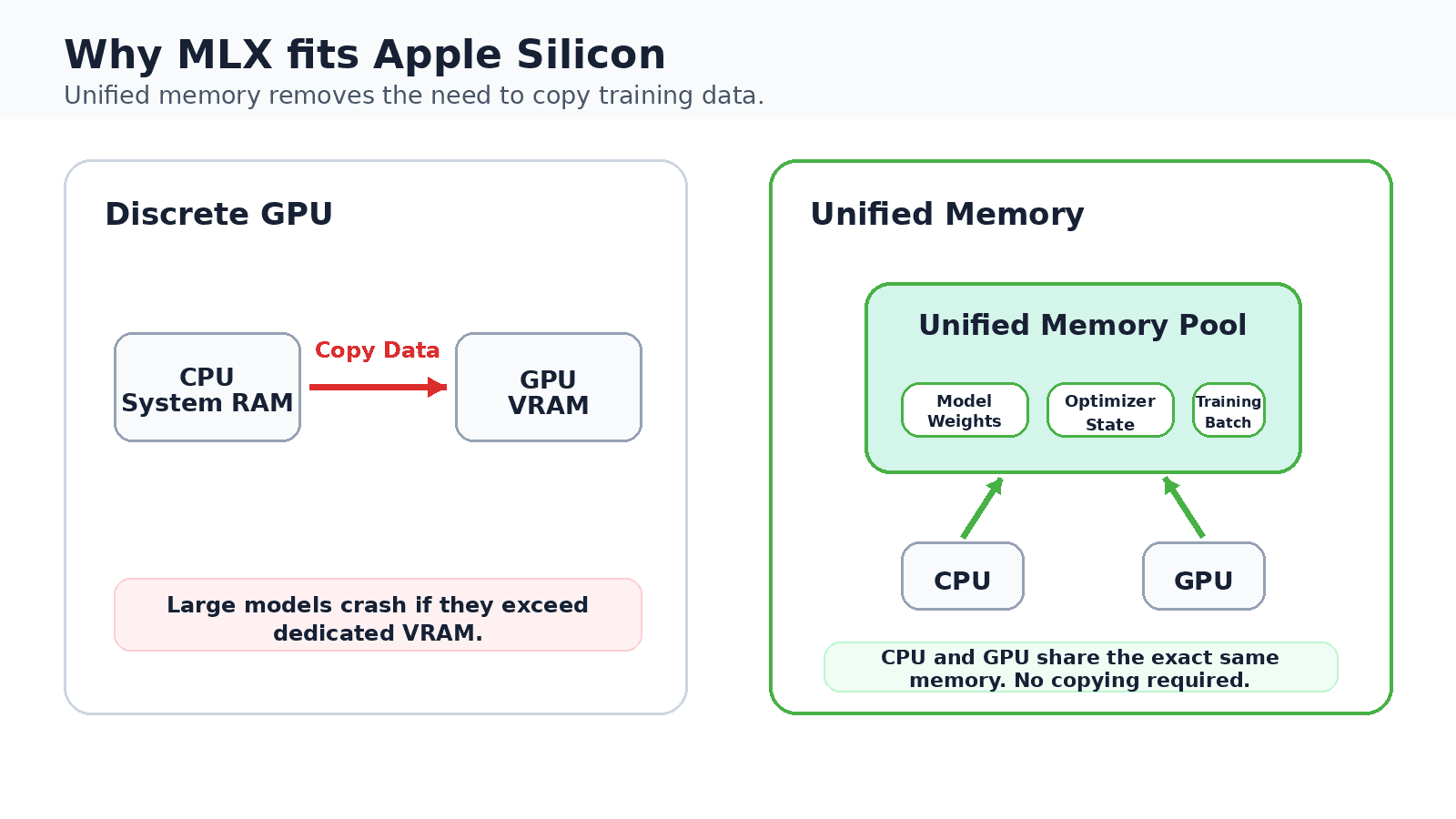
With a separate GPU, training data gets copied back and forth between system RAM and dedicated VRAM. Apple Silicon maintains a single shared pool, enabling a 16 GB Mac to fine-tune models entirely on-device.
# Getting Your Environment Ready
With that architectural advantage in mind, let’s install what you need. Begin with the core package along with its training extras, which automatically pulls in every dependency the fine-tuning commands require.
pip install "mlx-lm[train]"Check that everything installed correctly by running a quick generation test with a compact model.
mlx_lm.generate
--model mlx-community/Mistral-7B-Instruct-v0.3-4bit
--prompt "Explain LoRA in two sentences."
--max-tokens 120
The initial run fetches a 4-bit quantized Mistral model from the MLX Community group on Hugging Face, stores it locally, and then streams the output back to you. The mlx-community organization hosts thousands of pre-converted models, so you’ll rarely need to handle weight conversion yourself.
One important limitation to be aware of from the start: MLX fine-tuning only works with models stored in Hugging Face’s safetensors format. GGUF files, which are common in other local tools, are fine for inference but cannot be used for training. Compatible model architectures include Llama, Mistral, Qwen2, Phi, Gemma, and Mixtral, among others, so the majority of popular open models are supported right away.
# Structuring Your Dataset
With the environment prepared, the next task is getting your data into a format the trainer can consume. MLX LM expects training data inside a directory containing three files: train.jsonl, valid.jsonl, and an optional test.jsonl. Every line represents one JSON record. The training file is mandatory, the validation file allows the trainer to log validation loss during runs, and the test file is used to score the model after training is complete.
Three data formats are available: chat, completions, and text. The chat format is the most dependable default choice. It stores role-labeled messages on each line and allows MLX LM to apply the model’s native chat template, ensuring your data aligns with how the model was originally trained to process conversations.
{"messages": [{"role": "user", "content": "What is LoRA?"}, {"role": "assistant", "content": "An efficient way to fine-tune a model."}]}For straightforward input-output pairings, the completions format offers a simpler option and works nicely for instruction-based tasks.
{"prompt": "Summarize: The market rose sharply today.", "completion": "Markets gained."}
{"prompt": "Translate to French: good morning", "completion": "bonjour"}
By default, the trainer calculates loss across the entire example, which means the model devotes effort to reproducing both the prompt and the response. Using --mask-prompt directs it to compute loss only on the completion portion, so training hones in on the answer you actually want. This generally yields a model that follows instructions more consistently, and it’s compatible with both the chat and completions formats. When using chat data, the last message in the list is regarded as the completion.
Make sure each example occupies a single line with no embedded line breaks, because the reader interprets each line as an independent record. Allocate your data so that approximately 80 percent goes into train.jsonl and 10 to 20 percent into valid.jsonl. A practical lower bound for shifting a model’s behavior is around 200 to 500 examples (smaller sets tend to cause overfitting and memorization rather than real generalization).
# Training Your First LoRA Adapter
With your dataset ready is where things get exciting. Instead of updating every parameter in the model, Low-Rank Adaptation (LoRA) keeps the original weights frozen and trains compact adapter matrices alongside them. This slashes both memory and storage requirements to a small fraction of what full fine-tuning demands while preserving most of the quality. The method comes from
The LoRA paper, authored by Hu et al., introduced this parameter-efficient fine-tuning method.

LoRA keeps the large pretrained weights frozen and trains only the small matrices A and B. Because just those two adapters receive updates, memory and storage stay low.
Kick off a training session with a single command, supplying the path to a model and your data directory.
mlx_lm.lora
--model mlx-community/Mistral-7B-Instruct-v0.3-4bit
--train
--data ./data
--iters 600
--batch-size 1
During execution, MLX LM displays training loss, validation loss, tokens processed, and iterations per second. By default, adapter weights are written to an adapters folder. Several important flags to be aware of: --fine-tune-type takes lora (the default), dora, or full; --num-layers determines how many transformer layers get adapters (default: 16); and --iters governs training duration.
The example deliberately uses --batch-size 1 to minimize memory consumption. This helps avoid crashes on 16 GB machines. If you have 64 GB or more, bumping it up to 2 or 4 reduces overall training time. When memory is limited but you still want the stabilizing effect of a larger batch, --grad-accumulation-steps increases the effective batch size without adding to memory usage.
If you’d rather see live graphs than terminal output, include --report-to wandb to send metrics to Weights & Biases. If you run into memory pressure, drop --num-layers to 8 or 4, or add --grad-checkpoint to trade extra computation for reduced memory. These two options are typically sufficient to fit a job that would otherwise exceed available memory.
# Choosing a Base Model and Adapter Settings
Building on the training mechanics described above, two early choices shape everything that follows: which model to start from, and how much of it to adapt. For a first project, an 8B parameter model in 4-bit form hits the sweet spot. Once the workflow feels familiar, you can step up to 13B or 14B models, which require 14 to 18 GB of working memory and run comfortably on a 32 GB machine.
The number of trained layers and the adapter rank together determine capacity. More layers and a higher rank give the adapter greater ability to learn, at the expense of memory and time. A typical starting point uses 16 layers with a moderate rank, then adjusts depending on whether validation loss continues to decrease. If training loss falls while validation loss rises, the adapter is memorizing your examples rather than generalizing.
Learning rate also plays a key role. Values between 1e-5 and 5e-5 work well for most LoRA runs. Set it too high and training turns unstable; set it too low and the model barely changes. Adjust one setting at a time so you can trace any improvement back to a specific choice.
# Reducing Memory Use with Quantization
Notice that the base model above already ends in 4bit. Training a LoRA adapter on top of a quantized model is what people call QLoRA, as outlined in the QLoRA paper. Because quantization is built into MLX, the same mlx_lm.lora command trains adapters directly on quantized weights with no extra configuration needed.
The benefit is tangible. A 4-bit 7B model reduces weight memory by roughly 3.5 times compared with full precision, bringing a 7B fine-tune comfortably within 8 GB of working memory. On a 16 GB MacBook, that leaves plenty of headroom for the operating system and your training batch.
If you’d rather quantize a full precision model yourself before training, the convert command takes care of it.
mlx_lm.convert
--hf-path mistralai/Mistral-7B-Instruct-v0.3
--mlx-path ./mistral-4bit
-q
This writes a 4-bit version to a local folder that you then pass to --model.
# Testing and Generating with Your Adapter
With training finished, it’s time to evaluate how well the adapter learned. Score it against your held-out test set to obtain a number you can track across experiments.
mlx_lm.lora
--model mlx-community/Mistral-7B-Instruct-v0.3-4bit
--adapter-path ./adapters
--data ./data
--test
To see the model in action, pass the same adapter path to the generate command. MLX LM loads the base model and layers your adapter on top.
mlx_lm.generate
--model mlx-community/Mistral-7B-Instruct-v0.3-4bit
--adapter-path ./adapters
--prompt "Summarize: Our quarterly revenue grew twelve percent."
Run the same prompt without the adapter to compare. If your dataset matched the target task well, the adapted responses should follow your training examples more closely than the base model does.
# Fusing and Serving the Model
Adapters are handy during experimentation, but for deployment you often want a single, self-contained model. The fuse command merges the adapter back into the base weights.
mlx_lm.fuse
--model mlx-community/Mistral-7B-Instruct-v0.3-4bit
--adapter-path ./adapters
--save-path ./fused-model
The fused folder behaves like any other MLX model. You can serve it through an OpenAI-compatible endpoint, which lets existing client code talk to your local model after only a base URL change.
mlx_lm.server --model ./fused-model --port 8080
For a graphical alternative, LM Studio runs MLX models with a one-click local server and a chat interface, which is especially useful when you want to compare your fine-tuned model against others side by side.
# Wrapping Up
You now have a complete local fine-tuning workflow: install MLX LM, format a dataset as JSONL, train a LoRA or QLoRA adapter with a single command, test it, then fuse and serve the result. Everything runs on the Mac you already own, with no cloud bill and no data leaving your machine.
For me, this feels like a natural extension of the journey that began when I switched to Mac in 2014. The tight hardware-software integration that first drew me in has quietly evolved into something far more powerful, a machine capable of serious machine learning work at the kitchen table.
A few directions are worth exploring next. Try the dora fine-tune type and compare its results against plain LoRA. Adjust the number of trained layers and iteration count to balance quality against speed. Swap in a different base architecture. Llama, Qwen, Phi, and Gemma all work through the same commands. Each experiment is inexpensive when the hardware is sitting on your desk, which is the practical change MLX brings to adapting language models.
Vinod Chugani is an AI and data science educator who bridges the gap between emerging AI technologies and practical application for working professionals. His focus areas include agentic AI, machine learning applications, and automation workflows. Through his work as a technical mentor and instructor, Vinod has supported data professionals through skill development and career transitions. He brings analytical expertise from quantitative finance to his hands-on teaching approach. His content emphasizes actionable strategies and frameworks that professionals can apply immediately.