



# Evaluating Metric Calibration and Predictive Performance in Single-Cell Perturbation Modeling
Single-cell perturbation experiments have become a cornerstone of modern functional genomics, enabling researchers to measure how genetic or chemical interventions reshape cellular transcriptomes. As computational methods for predicting these responses mature, a critical question emerges: how do we reliably assess whether a model’s predictions are both accurate and well calibrated? This article provides a comprehensive overview of the baselines, metrics, and evaluation frameworks used to benchmark predictive models in this domain, drawing on a systematic study of 14 genetic perturbation datasets across diverse cell lines.
## Defining Meaningful Baselines
To contextualize model performance, it is essential to establish baselines that range from trivially simple to near-perfect. These baselines help distinguish genuine predictive signal from noise or dataset structure.
### The Control Baseline
The control baseline, denoted as μc, is the averaged expression profile of a large set of unperturbed control cells. At the dataset level, this serves as a reference representing the unperturbed state. Predictions are evaluated against this baseline to capture how well a model recovers the shift induced by a perturbation relative to a null hypothesis of no change.
### The Mean Baseline
The mean baseline, μall, is computed as the average of all training perturbation profiles, with each perturbation contributing equally regardless of its cell count. Mathematically, it is the mean of the per-perturbation averages. This baseline represents a dense, equally weighted estimate of the average perturbation effect across the training set, providing a simple but powerful reference for evaluating whether a model can outperform a dataset-wide average.
### The Technical Duplicate Baseline
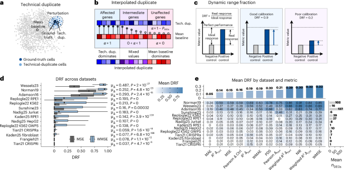
The technical duplicate baseline offers an idealized estimate of performance where the only source of error is inherent biological or technical variability within the same perturbation. To construct it, the cells associated with each perturbation are randomly split into two halves: a ground-truth set and a technical-duplicate set. The average profile of the technical-duplicate set serves as the prediction, and the average profile of the ground-truth set serves as the target. This setup answers a practical question: if we sequenced additional cells from the same perturbed sample, how predictive would they be of the effect originally observed? Because the prediction and ground truth come from the same perturbation, this baseline is not susceptible to data leakage when used for calibration assessment, provided that the technical-duplicate cells are excluded from all downstream weight or mask computations.
### The Interpolated Duplicate Baseline
The interpolated duplicate refines the technical duplicate by incorporating a confidence-weighted blend between the technical-duplicate prediction and the mean baseline. For each gene, an interpolation weight α is derived from the statistical significance of differential expression, computed exclusively on the held-out technical-duplicate half of the perturbation. When a gene is strongly affected by a perturbation, α approaches 1, and the prediction relies on the technical duplicate. When a gene is unaffected, α approaches 0, and the prediction reverts to the mean baseline. This produces an interpretable, per-gene confidence measure that bounds interpolation weights between 0 and 1.
### The Linear Baseline
The linear baseline is a deliberately simple model that uses principal component analysis (PCA) to capture the dominant axes of variation in the pseudobulked training data. After projecting the data onto a principal component matrix, a ridge regression is fit to predict perturbation effects from a small number of latent components. Predictions for unseen perturbations are obtained by transforming the new perturbation’s representation through the learned linear mapping. This baseline is evaluated exclusively on unseen single perturbations and serves as a sanity check for more complex models.
### The Additive Baseline
For combination perturbation tasks, the additive baseline predicts the effect of two perturbations combined by summing their individual effect profiles and subtracting the control baseline. This simple assumption of independence provides a reference point for evaluating models that attempt to capture interaction effects between perturbations.
## Data Processing and Experimental Design
The evaluation framework draws on a heterogeneous collection of genetic perturbation datasets, spanning multiple cell lines and both activation and repression perturbations. All datasets undergo a standardized processing pipeline: low-quality cells and genes are filtered, library sizes are normalized, and log transformation is applied. To ensure balanced evaluation, each perturbation is capped at a maximum cell count, and a gene set comprising the top highly variable genes plus all perturbed genes is retained for analysis.
A key aspect of the design is the construction of technical duplicates. Before any cross-validation, the cells for each perturbation are randomly split once into ground-truth and technical-duplicate halves. This split is fixed across all folds. During training, both halves are available for perturbations assigned to the training set, but during testing, neither half is observed. At evaluation time, the ground-truth half defines the true target, while the technical-duplicate half is reserved exclusively for baseline construction. This mirroring ensures that the same data splitting logic applies to both model evaluation and baseline calibration, preventing information leakage.
Differential expression analysis is performed separately on each half of each perturbation against all other perturbed cells, deliberately excluding control populations. This design focuses evaluation on genes that make a given perturbation unique, rather than on genes that change universally across all perturbations.
## Metric Calibration: Measuring the Reliability of Evaluation Metrics
A metric can be accurate yet poorly calibrated if it fails to translate prediction quality into a meaningful score. To assess calibration, the authors introduce the Delta Reference Fraction (DRF), which quantifies how much of the ideal performance gap between a perfect predictor and a negative control is actually achieved by a real predictor. Formally, DRF is the ratio of the score difference between the positive control (ideal prediction) and the negative control (naïve baseline) to the score difference between the ground truth and the negative control. A DRF of 1 indicates perfect calibration; a DRF near 0 suggests the metric fails to distinguish signal from noise.
In this framework, the ground truth is the technical-duplicate average, the positive control is the interpolated duplicate, and the negative control is the mean baseline. The DRF is computed per perturbation, enabling analysis of how calibration varies across factors such as perturbation strength, gene set size, and sequencing depth.
## A Suite of Complementary Evaluation Metrics
Different applications demand different aspects of predictive accuracy. The evaluation suite spans four categories to capture a holistic picture of model performance.
### Direct Error Metrics
Mean squared error (MSE) and mean absolute error (MAE) measure the raw reconstruction error between predicted and observed expression profiles. Weighted versions—WMSE and weighted MAE—apply gene-level importance scores derived from differential expression, emphasizing errors in genes that are most strongly affected by the perturbation. These weighted metrics are particularly relevant for applications where the goal is to detect subtle but biologically meaningful changes in specific pathways or gene modules.
### Reference-Based Delta Metrics
Delta-based metrics assess whether a model captures the direction and relative magnitude of perturbation-induced changes by comparing the predicted shift against a reference baseline. Common choices include Pearson correlation and the coefficient of determination R², computed relative to either the control cell average or the perturbed mean baseline. Because correlation alone does not penalize differences in scale, R² is included to provide a more comprehensive assessment of fit. For metrics where the reference and predictor coincide (such as the control baseline’s Pearson delta), the evaluation is undefined and is either substituted with an alternative negative control or excluded from summaries.
### Retrieval-Based Metrics
Retrieval-based metrics evaluate the global relational structure of the prediction space. The normalized inverted rank (NIR) and perturbation discrimination score (PDS) assess whether a model’s predicted profile is most similar to its correct ground-truth perturbation relative to all other perturbations. These metrics use Euclidean (L2) or Manhattan (L1) distance, respectively, and are crucial for applications like network inference, where preserving the neighborhood relationships among perturbations matters as much as per-gene accuracy.
### DEG-Based Metrics
For applications focused on specific genes or pathways, performance is evaluated exclusively on the top differentially expressed genes per perturbation. After ranking genes by adjusted P value, standard error and delta metrics are computed over this subset. Because the feature space is restricted, these metrics are analyzed separately from genome-wide evaluations, providing insight into a model’s ability to prioritize biologically relevant genes.
## Sensitivity to Experimental Parameters
The reliability of metric calibration can depend on the experimental design itself. To investigate this, a series of sensitivity analyses were conducted on a dataset with strong overall calibration and high cell counts per perturbation.
### Cell Count Sensitivity
By downsampling cells per perturbation to a range of target counts, the analysis reveals how calibration degrades as per-perturbation sample sizes shrink. At each cell count, all baselines and metrics are recomputed, and the DRF for each metric is tracked. This allows researchers to understand the minimum cell numbers required for a metric to remain informative and to interpret calibration results in the context of their own experimental design.
### UMI Depth Sensitivity
Sequencing depth varies across experiments and can introduce systematic biases. In the UMI downsampling analysis, cells are filtered for high total UMI counts, and the number of UMIs per cell is reduced to a range of target depths while keeping the total cell count fixed. At each depth, all preprocessing steps—including normalization, highly variable gene selection, and differential expression—are repeated independently. The resulting DRF values show how calibration depends on sequencing depth and highlight the importance of adequate coverage per cell.
### Highly Variable Gene Selection Sensitivity
The choice of how many highly variable genes to retain can influence both model training and metric computation. By sweeping the number of top HVGs from a small set to the full gene set, the analysis examines how gene variance filtering affects calibration. Each gene count threshold triggers a fresh round of differential expression and baseline recomputation, isolating the impact of feature space selection on metric reliability.
## Biological Signal Validation
Beyond statistical metrics, it is valuable to assess whether models preserve known biological relationships. Two complementary analyses serve this purpose.
### Transcription Factor Enrichment
A gene set enrichment analysis is performed to identify transcription factors whose target genes are differentially expressed in response to specific perturbations. Using overlapping perturbations from a well-characterized dataset, the analysis ranks TFs by the strength of their self-enrichment signals. Selecting TFs with few significant DEGs but strong enrichment highlights cases where models can recover focused regulatory programs, even when the overall transcriptomic shift is modest.
### Pathway Recovery
To evaluate whether predictions capture pathway-level biology, gene set enrichment is performed on the predicted and ground-truth expression shifts for each test perturbation. The enrichment results for the 50 Hallmark pathways are compared using Pearson correlation between the two normalized enrichment score vectors. A high correlation indicates that the model correctly predicts which pathways are activated or repressed, even if individual gene predictions are noisy. This captures a form of global biological fidelity that pointwise accuracy metrics alone cannot assess.
### Neighborhood Recovery
A complementary analysis evaluates the preservation of local perturbation relationships. K-nearest-neighbor graphs are constructed from the expression shifts of all test perturbations, one built from ground truth and one from predictions. The agreement between the two ranked neighbor lists is quantified using rank-biased overlap, a metric that weighs top matches more heavily. High overlap indicates that the model places perturbations in a similar neighborhood structure as the ground truth, preserving the geometry of the perturbation response landscape.
## Benchmarking Deep Learning Models
To determine whether strong calibration and performance results generalize across architectures, a diverse set of deep learning models was benchmarked. The suite includes transformer-based models like scGPT, graph neural networks such as GEARS, variational autoencoders with large language model-derived embeddings, flow-matching generative models like CellFlow, and delta-predicting models like PRESAGE. All models were implemented as close to their original versions as possible, with minimal modifications necessary for benchmarking, and were evaluated under consistent cross-validation schemes.
In addition to off-the-shelf models, the study employs a probing strategy using multi-layer perceptrons (fMLPs) trained on perturbation embeddings extracted from foundation models such as Geneformer, GenePT, ESM2, and scGPT. This approach isolates the contribution of the perturbation representation from the model architecture, allowing a direct test of whether foundation models capture useful perturbation information. A size ablation over the fMLP further tests whether performance gains are driven by representational quality or simply by increased model capacity.
## Benchmark Setup and Statistical Rigor
Model evaluation uses fivefold cross-validation for unseen single perturbations and twofold cross-validation for unseen combination perturbations. Within each fold, cells from technical duplicates are treated as held-out data for both baselines and models. All evaluation metrics are computed on perturbation-level pseudobulk profiles to ensure comparability. Statistical comparisons between models and baselines are performed using paired tests with Bonferroni correction for multiple comparisons. Effect sizes are reported alongside confidence intervals derived from bootstrapping, ensuring that conclusions are robust and reproducible.
## FAQ: Understanding Metric Calibration and Benchmarking
**Q: Why do we need so many different evaluation metrics?**
A: Different downstream applications rely on different aspects of predictive accuracy. A model might excel at reconstructing the full transcriptome but fail to capture pathway-level signals, or it might rank genes well but produce poorly calibrated expression values. Using a diverse suite of metrics ensures a more complete picture of where a model succeeds or struggles.
**Q: What does it mean for a metric to be “calibrated”?**
A: Calibration refers to the alignment between a metric’s output and the true quality of a prediction. A well-calibrated metric should assign higher scores to better predictions and lower scores to worse ones, relative to a known perfect predictor and a negative control. A metric can have high discriminatory power yet be poorly calibrated if it saturates or is insensitive to differences in prediction quality.
**Q: How does the technical duplicate baseline prevent data leakage?**
A: The technical duplicate baseline uses a random split of cells within each perturbation into two independent halves. During model training, both halves are available for training perturbations. During testing and baseline construction, only the appropriate half is used, and the technical-duplicate cells are never used to compute evaluation weights or DEG masks. This ensures that the baseline is constructed from data the model has never seen in the evaluation context.
**Q: What is the purpose of the interpolated duplicate baseline?**
A: The interpolated duplicate blends the technical-duplicate prediction with the mean baseline using a gene-specific weight derived from differential expression significance. This produces a prediction that uses the technical-duplicate when there is strong evidence a gene is perturbed and falls back to the mean baseline for unaffected genes. It serves as a near-ideal positive control for calibration because it leverages ground-truth statistical evidence to guide predictions.
**Q: How are combination perturbations handled in the benchmark?**
A: Combination perturbations are evaluated in a separate unseen combination task. During training, all single perturbations are available, while double perturbations are split into training and test sets. The additive baseline provides a simple independence assumption against which models that attempt to learn interaction effects can be compared.
**Q: Why is pathway recovery important if individual gene predictions are noisy?**
A: Biological pathways are often regulated by coordinated, weak signals across many genes. A model may not accurately predict every gene’s expression but still capture the aggregate activation or repression of a pathway. Pathway recovery metrics assess this global biological fidelity, which can be more relevant for downstream interpretation than per-gene accuracy.
**Q: What did the sensitivity analyses reveal about metric reliability?**
A: The analyses showed that calibration and metric performance degrade as cell counts, sequencing depth, and the number of highly variable genes decrease. This highlights the importance of having sufficient data per perturbation and appropriate filtering, and it offers guidance for interpreting benchmark results in the context of limited or noisy datasets.
## Conclusion
Rigorous benchmarking of single-cell perturbation models requires more than a single accuracy metric. It demands a principled set of baselines that span the range from trivial to ideal, a careful framework for metric calibration that distinguishes signal from noise, and a diverse evaluation suite that captures multiple facets of biological relevance. By combining direct error metrics, delta-based comparisons, retrieval-oriented structural assessments, and gene-level filtering, researchers can gain a nuanced understanding of model strengths and weaknesses. The sensitivity analyses further underscore that the reliability of these metrics depends on experimental design choices such as cell count, sequencing depth, and gene filtering. As the field continues to develop more sophisticated models, this comprehensive evaluation paradigm provides a blueprint for honest, reproducible assessment and for identifying where current methods succeed—and where they still fall short—in capturing the complexity of the cellular response to genetic and chemical perturbations.
Thank you for reading
