



# Do Autoencoders Actually Beat PCA for Anomaly Detection? A Practical Investigation
## The Promise of Autoencoders
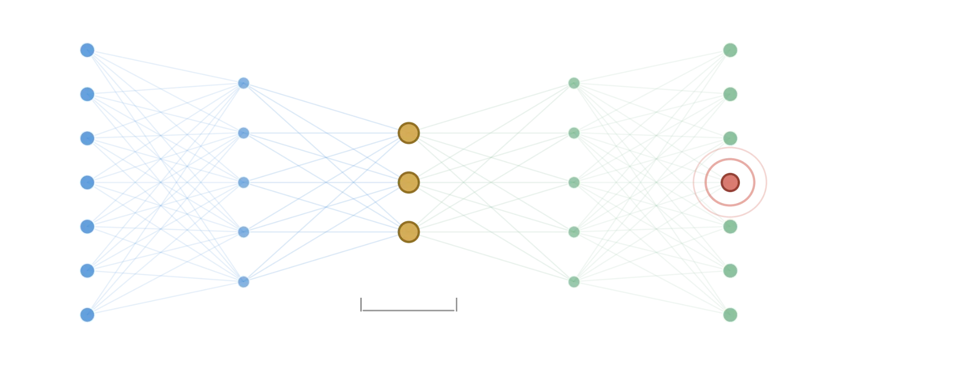
Autoencoders are neural networks designed to compress input data into a smaller latent representation and then reconstruct it back to the original dimensions. When trained exclusively on normal, unlabeled data, they develop an internal model of what “regular” patterns look like. The underlying logic for using them in anomaly detection is straightforward: during inference, data points that deviate from learned patterns produce high reconstruction errors, which can then be flagged as potential outliers.
This stands in contrast to Principal Component Analysis (PCA), a linear dimensionality-reduction technique that also serves as a baseline for reconstruction-based anomaly detection. PCA can only model linear correlations among features, whereas autoencoders — depending on their architecture — can theoretically capture complex, nonlinear dependencies. That raises a compelling hypothesis: if the normal data contains nonlinear structures that a linear method structurally cannot represent, then an autoencoder should demonstrate a measurable performance edge.
But does it actually pan out in practice? To find out, two controlled experiments were designed, comparing a default autoencoder architecture against PCA — both using the same latent dimensionality — along with Isolation Forest as a non-reconstruction-based reference point. All training was done on normal-only samples, with a held-out test set containing both normal and anomalous instances.
—
## The Experimental Design
Both experiments used synthetic datasets with clear labels, allowing for precise measurement of detection performance. The autoencoder was built using a shallow multilayer perceptron regressor trained to reproduce its own input, configured with a three-dimensional bottleneck to match the three principal components used in PCA. Reconstruction error — measured as mean squared error across features — served as the anomaly scoring mechanism for both reconstruction-based methods.
Performance was evaluated using the F1 score, which balances precision and recall, since anomaly detection tasks often deal with imbalanced class distributions where accuracy alone can be misleading.
—
## Experiment One: The Straightforward Case
In the first scenario, normal data was generated from a mixture of Gaussian clusters — simulating several distinct operating regimes of a system. Anomalous data was drawn from a distribution with a shifted center and increased spread, creating outliers that are separable by a linear boundary.
The results showed a near-perfect tie: both the autoencoder and PCA achieved an F1 score of approximately 0.885, successfully identifying every anomalous instance with perfect recall. Isolation Forest trailed slightly behind with an F1 of roughly 0.870.
The reconstruction error distributions revealed why this task was so simple for both methods. Normal samples clustered tightly below a reconstruction error of 1.0, while anomalous samples sat almost entirely above 4.0. With such a wide, clean gap between the two distributions, any reasonable decision threshold would perform well — which explains why the more powerful nonlinear model offered no advantage. When the signal is strong and linearly separable, adding complexity buys nothing.
—
## Experiment Two: Constructing a Challenge That Favors Nonlinearity
The second experiment was deliberately crafted to test the theoretical claim. Normal data included two features linked by a nonlinear relationship — specifically, one feature followed a sine curve relative to the other, with modest noise added. Anomalies preserved the same individual ranges for each feature but broke the dependency between them by drawing values independently, so that each variable looked normal in isolation while their joint combination was impossible under the learned normal pattern.
This construction is, in principle, a worst-case scenario for PCA: a linear projection genuinely cannot represent a curved manifold in feature space. If the autoencoder’s theoretical advantage is real, it should emerge here.
It did not.
PCA achieved an F1 score of 0.318, while the autoencoder scored 0.302 — a negligible difference with PCA holding a slight lead. Both methods performed substantially worse than Experiment One, reflecting the inherent difficulty of the task. Isolation Forest collapsed to an F1 of roughly 0.091, confirming that this was a genuinely hard problem for reconstruction-based methods across the board.
The reconstruction error histogram for this experiment told the real story: normal and anomalous samples overlapped heavily, with no clean threshold dividing them. Some anomalies produced lower reconstruction errors than perfectly normal samples, meaning that the detection signal itself — not just the choice of algorithm — was insufficient for clean separation. This is an important distinction: the problem was not that a particular method failed, but that the error surface did not provide a useful discriminative signal for either linear or nonlinear reconstruction.
—
## Why the Theoretical Edge Failed to Materialize
These results do not disprove the theoretical capacity of autoencoders to outperform linear methods. Rather, they reveal a gap between that capacity and what a default configuration actually delivers. Several factors likely contributed:
**Limited training data.** A neural network needs substantially more examples than a closed-form linear solution to learn a nonlinear manifold reliably. Seven hundred training samples may be sufficient for PCA to estimate its principal components accurately, but it is a small dataset for a neural network to discover a meaningful curved structure without overfitting or settling for a suboptimal solution.
**No hyperparameter tuning.** The autoencoder used a single, unsearch architecture (8–3–8 layers) with default training settings. Capturing a specific nonlinear relationship effectively often requires deliberate choices about depth, width, activation functions, and training duration — none of which were explored in this comparison.
**Signal dilution in reconstruction error.** When the anomalous signal lives in only a subset of features and is averaged across all dimensions during reconstruction, both linear and nonlinear methods can fail to amplify that signal sufficiently. This is a known structural weakness of global reconstruction error as an anomaly metric, and it affects neural networks and linear models alike.
—
## What Would It Take to Unlock the Advantage?
If the nonlinear signal is genuine, several practical steps can help an autoencoder realize its potential:
– **More training data.** Increasing the volume of normal samples gives the network more examples from which to learn the manifold, reducing the risk of the model fitting noise instead of signal.
– **Architectural customization.** Designing the network around the known structure of the problem — for instance, dedicating more capacity to the two features carrying the nonlinear relationship — can guide learning toward the relevant patterns.
– **Inspecting the latent space directly.** Visualizing the bottleneck activations colored by true labels can reveal whether the anomalies are separable at the representation level, distinguishing between a representation learning failure and a thresholding problem.
– **Weighted reconstruction loss.** Applying higher weights to the informative features prevents uninformative dimensions from diluting the anomaly signal in the overall error score.
None of these interventions are exotic; they represent the actual engineering effort that “just use a neural network” tends to skip.
—
## A Decision Framework Before Choosing Your Method
Before defaulting to an autoencoder over a simpler reconstruction-based method, three diagnostic questions are worth answering:
1. **Does the data actually contain nonlinear relationships, or does it merely appear complex?** Many datasets that feel like they should require a neural network are well-approximated by linear structures. Verifying the presence of genuine nonlinear dependencies — through visualization or statistical tests — is a necessary prerequisite before committing to a more complex model.
2. **Is there enough normal-only data for a neural network to learn reliably?** PCA’s linear solution is inherently data-efficient, requiring only enough samples to estimate covariance. Neural networks need substantially more data to avoid memorizing noise or failing to converge on a meaningful manifold.
3. **Have you inspected the reconstruction error distribution before committing to a threshold?** A simple histogram of reconstruction errors for both normal and anomalous samples, generated in minutes, immediately reveals whether the chosen method produces a usable discriminative signal at all. If the distributions overlap heavily regardless of method, the problem likely requires a fundamentally different approach rather than a different algorithm.
—
## Limitations of This Comparison
Several caveats apply to the findings presented here. The experiments used synthetically generated data rather than real-world sensor readings or transactional records, which means the exact numerical results may not transfer directly to production settings. Only one architecture and one training run were evaluated per method, which was intentional — this investigation focused on default configurations rather than optimized ones, but it means the ceiling of autoencoder performance remains unexplored. The anomaly generation used a single random seed, and different constructions could shift the specific outcomes, though the broader direction — no automatic advantage for the more complex model — appears robust.
—
## Frequently Asked Questions
**Q: Does this mean autoencoders are bad for anomaly detection?**
A: No. These results show that a default, untuned autoencoder does not automatically outperform PCA — not that autoencoders are ineffective. When properly configured with sufficient data, appropriate architecture, and thoughtful loss weighting, autoencoders can capture nonlinear patterns that linear methods miss. The takeaway is that the theoretical advantage requires deliberate engineering to realize.
**Q: Why use PCA at all if it’s a linear method?**
A: PCA is extremely data-efficient, computationally lightweight, and requires no hyperparameter tuning beyond the number of components. In many real-world scenarios, linear methods perform surprisingly well because the dominant patterns in tabular data are often approximately linear, or because the anomaly signal is strong enough to be detected even with a simplified model. Starting with PCA as a baseline and only escalating to neural networks when it demonstrably underperforms is a sound engineering practice.
**Q: What about unsupervised neural networks other than autoencoders?**
A: Variational autoencoders, generative adversarial networks, and diffusion models all offer different inductive biases for modeling normal data. The core lesson here — that representational capacity alone does not guarantee practical superiority — applies broadly to all of them. Each introduces additional complexity (more hyperparameters, more data requirements, more training instability), which raises the bar for realizing any advantage.
**Q: How much data is “enough” for an autoencoder to outperform PCA?**
A: There is no universal threshold, but the general guidance is that neural networks require an order of magnitude more samples than the number of trainable parameters to learn reliably. For the kinds of nonlinear manifolds tested here, thousands of samples are likely a more realistic starting point than hundreds. Domain-specific experimentation is essential — the histogram of reconstruction errors is your best diagnostic tool for knowing when you have crossed that line.
**Q: What if my anomalies are subtle and not linearly separable?**
A: Subtle anomalies in high-dimensional settings pose challenges for any reconstruction-based method. If both PCA and autoencoders produce heavily overlapping error distributions, the issue may be that the anomaly signal is too diffuse across features for global reconstruction error to capture it. In such cases, feature-specific scoring, supervised approaches (if any labels are available), or entirely different paradigms like density estimation or contrastive learning may be worth exploring.
—
## Conclusion
The ability of autoencoders to represent nonlinear relationships is a mathematical fact — but mathematical possibility and practical performance are two different things. This investigation demonstrated that a default autoencoder configuration, given limited data and no hyperparameter optimization, failed to outperform a simple linear baseline on a task specifically designed to test its theoretical advantage. The gap between what a model *can* do and what it *does* do is where the real engineering work lies.
The most important habit in applied machine learning is measuring before assuming. Before reaching for a more complex model, asking whether the improvement shows up in a controlled, measurable comparison — rather than only in theory — prevents wasted effort and leads to more robust systems. The simplest method that meets the requirement is often the right choice, and escalating to neural networks should be a deliberate decision backed by evidence, not a reflex.
Thank you for reading
