



# Why Averaging Neural Network Weights Often Fails — And What to Do About It
## The Puzzle of Two Identical Training Runs
Imagine training the same neural network architecture twice on the same dataset. You change nothing except the random seed. Both runs converge. Both achieve the same training loss. You would be forgiven for assuming the results are interchangeable — that averaging their weight vectors should give you a model at least as good as either one alone.
In practice, the average is frequently worse. Much worse.
This is not a training bug, not a hyperparameter mishap, and not evidence of instability. It is a structural property of neural networks, rooted in a concept called **permutation symmetry**. Understanding this symmetry also explains why some model merging strategies succeed while others fail — a question that sits at the core of modern model engineering, from model soups to federated learning aggregation.
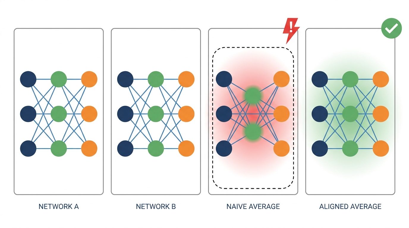
Before diving into the mathematics, here is a way to build intuition: imagine two trained networks as two spreadsheets describing the same report, but with their columns shuffled into a different order. Spreadsheet A’s “column 3” might correspond to spreadsheet B’s “column 7.” Both spreadsheets are correct, both produce the same totals, but if you average them cell by cell without first reconciling the column order, you end up mixing revenue figures with headcounts. That is exactly what naive weight averaging does to a neural network.
This article explores the geometry of neural network solutions — what the set of good models actually looks like — rather than focusing on what functions the network computes.
—
## Why Neural Networks Are Inherently Non-Convex
Many classical machine learning models follow a simple template:
**f(x) = Σ aᵢ · ϕᵢ(x)**
Here, **ϕᵢ(x)** represents a fixed set of basis functions, and **a** is a vector of coefficients. Polynomial regression, for example, uses ϕ₁(x) = 1, ϕ₂(x) = x, ϕ₃(x) = x², and so on. Kernel ridge regression uses an implicit, effectively infinite basis defined by a kernel function. In both cases, only the coefficients are learned, and the resulting optimization problem is convex — there is one global minimum, a closed-form solution, and no dependence on random initialization.
Neural networks change one crucial element: the basis functions themselves are learned. Each neuron acts as an adaptive basis function, and the network simultaneously learns both the basis and the coefficients by minimizing a squared-error-style loss.
This single shift is the origin of everything that follows. **Non-convexity is not an accident of any particular activation function — it is the price of adaptivity.** If you fix the basis, you retain convexity. If you let the network learn the basis, you lose it. There is no middle ground.
And with that loss of convexity comes the “column ordering” problem. In polynomial regression, the columns are fixed by convention: x, x², x³, in that agreed-upon order. In a neural network, the columns are learned alongside everything else. There is no pre-established convention dictating which neuron should occupy which position. That absence of a canonical ordering is the complete origin of permutation symmetry.
—
## The Geometry of Symmetry: How Permutation Creates Identical Solutions
Consider a minimal example: a network with two neurons, one input, and ReLU activations:
**f(x) = ReLU(x − w₁) + ReLU(x − w₂)**
The loss function treats w₁ and w₂ interchangeably. Swapping their values produces exactly the same function and therefore the same loss. If (w₁, w₂) is a global minimum, then (w₂, w₁) is equally valid.
Now consider the midpoint between these two minima: ((w₁ + w₂)/2, (w₁ + w₂)/2). Both neurons have identical parameters, which means the network effectively has the capacity of a single neuron, not two. Unless one of the original neurons was doing nothing at all, this midpoint cannot be optimal.
This reveals something profound about the loss landscape: it is not merely bumpy — it contains **exact copies of the same valley**, separated by barriers. For a hidden layer with **m** units, there are **m!** equivalent orderings. A layer with 512 neurons gives approximately 512! ≈ 10¹¹⁶⁶ copies of every solution. That is 512 factorial different ways to shuffle the same set of columns — each one an equally valid representation of the same underlying function.
—
## A Concrete Two-Neuron Demonstration
To make this tangible, consider a simple experiment. Two neurons and one input create a landscape that can be fully visualized. Taking the ground truth weights w = (2, 6) and generating 200 data points with Gaussian noise, we can plot the loss surface and observe the symmetry firsthand.
The global minima arrive in mirror-image pairs: (2, 6) and (6, 2) both yield the same loss. The surface is perfectly symmetric about the diagonal line where w₁ = w₂, because that diagonal is the set of points unchanged by swapping the two neurons.
The straight-line path connecting the two minima climbs sharply. At the midpoint (4, 4), the loss is roughly **6.4 times higher** than at either minimum. This elevation is the barrier between equivalent basins — the same quantity studied in the linear mode connectivity literature, made visible in two dimensions.
Which minimum a training run settles into is essentially a coin flip. Running gradient descent from 40 random starting points yields roughly 47% convergence to one ordering and 53% to the other. The random seed picks the basin; nothing else does.
### What Happens When You Merge Without Alignment
Train two models from different random starts and compare their weights:
| Configuration | w₁ | w₂ | Loss |
|—|—|—|—|
| Model A | ~2.0 | ~6.1 | ~0.09 |
| Model B | ~6.1 | ~2.0 | ~0.09 |
| Naive average of A and B | ~4.0 | ~4.0 | ~0.60 |
| Average after reordering B to match A | ~2.0 | ~6.1 | ~0.09 |
The naive average is dramatically worse — roughly **6.5 times the loss** of either input model. But once you reorder Model B’s neurons to align with Model A’s, the simple average snaps back to a model with identical performance. Nothing about what Model B computes has changed. Only the labels assigned to its neurons have been corrected.
—
## The Same Principles at Larger Scale
The two-neuron picture generalizes surprisingly well. Research has shown that most stochastic gradient descent solutions land in the same basin **once permutation symmetry is taken into account**. Algorithms designed to find the correct aligning permutation between models have demonstrated that independently trained deep networks — including ResNets on benchmark datasets — can be merged with near-zero loss penalty, provided the hidden units are first relabeled to match.
That said, the caveats are meaningful. Zero-barrier connectivity after alignment has been observed primarily in sufficiently wide networks; narrower architectures often retain barriers between basins. The width of the network appears to be a key factor in determining whether clean merging is possible. Additionally, some research suggests that activation statistics may also need correction after interpolation, beyond simple permutation alignment.
—
## Five Practical Principles for Weight Averaging and Model Merging
The geometry described above gives rise to several concrete rules:
### 1. Model soups work best when models share a common ancestor
Checkpoints derived from the same pre-trained base tend to remain within the same basin. Averaging them without alignment often succeeds in these cases. However, if fine-tuning procedures differ significantly — in learning rate, regularization strength, or training duration — the resulting models may occupy different basins, and naive averaging will degrade performance. Always inspect the interpolation curve before committing to an average.
### 2. Merging unrelated models requires an alignment step first
Techniques such as permutation-based alignment algorithms and activation-statistics correction have become standard preprocessing steps before performing task arithmetic or other merging operations. Skipping alignment when models have been trained independently is the single most common cause of merging failures.
### 3. Distance in weight space does not measure model similarity
Two networks that are functionally identical can be very far apart in ℓ₂ distance — especially when continuous symmetries like rescaling are present, since the labels assigned to neurons are arbitrary. When tracking training drift or comparing models, use representation-level metrics such as centering kernel alignment (CKA) or output agreement on a held-out validation set instead of raw parameter distance.
### 4. Ensembles are safest when built in function space, not parameter space
Averaging predictions is permutation-invariant by construction. Averaging weights is not. This is precisely why deep ensembles — where each model contributes a prediction — tend to outperform weight-averaged models when the constituent models are trained independently.
### 5. Bayesian posteriors over weights are naturally multimodal
A posterior distribution over the weights of a layer with m units has at least m! identical modes. Approximating this posterior with a single Gaussian (as mean-field variational inference does) fundamentally misses this structure. This is one reason such approximations underestimate uncertainty. Deep ensembles work in part because independent training runs sample different symmetry-equivalent modes of the same posterior.
—
## Beyond Permutation: Other Symmetries You Should Know
Permutation symmetry is powerful, but it is not the only symmetry lurking in neural networks. ReLU networks exhibit **positive-rescaling symmetry**: you can scale a neuron’s incoming weights and bias by a positive constant c, and its outgoing weights by 1/c, leaving the function unchanged — because ReLU(cz) = c · ReLU(z) for c > 0. This is analogous to having two columns in a spreadsheet that represent the same information in different units (dollars vs. cents). No reordering will detect it, because nothing has moved; everything has only been rescaled.
Transformer architectures introduce even more complexity. Recent work has shown that **rotational invariances** among attention heads matter when fusing transformer models, because attention heads possess symmetries that simple unit relabeling does not capture.
The unifying message across all of these symmetries is the same: **the parameters are coordinates of a function, not the function itself.** Many different coordinate systems describe the same point in function space. Any merging or averaging procedure must account for this before combining weights.
—
## A Minimal Alignment Implementation
For practitioners who want to experiment with permutation alignment, here is a straightforward approach using NumPy and SciPy. The idea is to match hidden units between two models based on how similarly they respond to the same inputs, then reorder one model’s units to correspond to the other’s.
The process works as follows:
1. Train two single-hidden-layer models from different random seeds on the same data.
2. Pass a representative batch of inputs through both models to collect hidden-layer activations.
3. Compute the correlation matrix between each pair of hidden units across the two models.
4. Use the Hungarian algorithm to find the permutation of Model B’s units that maximizes total alignment with Model A’s units.
5. Reorder Model B’s weight matrices according to this permutation.
6. Average the aligned weights and evaluate the merged model.
This approach generalizes the core idea to any architecture with a distinguishable hidden layer, and it can be adapted for deeper networks by aligning layer by layer.
—
## Important Caveats and Limitations
Before applying these ideas in production, keep a few nuances in mind:
– **Zero-barrier connectivity after alignment is not guaranteed.** The theoretical conjecture that most solutions are connectable by near-zero-loss paths after permutation alignment holds well for wide networks but not universally. Narrow architectures, different training setups, and certain data distributions may still exhibit significant barriers.
– **Permutation is not the only source of non-convexity.** While symmetry accounts for a large, well-characterized portion of the non-convex landscape, optimization geometry, network depth, data geometry, and training dynamics all contribute as well. Merging failures can stem from feature mismatch, activation distribution shifts, width mismatches, and other factors beyond permutation alone.
– **The random seed is not the only determinant of which basin you land in.** Architecture width, learning rate, batch ordering, optimizer choice, and data ordering all influence which symmetry-equivalent basin gradient descent finds.
– **Symmetry is sufficient to create non-convexity, but it may not explain all of it.** “Most non-convexity comes from symmetry” is a well-supported hypothesis and a productive organizing principle, not a proven theorem that covers every case.
—
## FAQ
**Q: Does this mean I should never average neural network weights directly?**
A: Not necessarily. If the models being averaged come from the same training run (e.g., snapshots taken during a single training process), they are typically in the same basin and averaging works well. The failure mode appears when averaging models trained independently from different seeds without first aligning them. The key question is whether the models share a common training trajectory.
**Q: Is model merging the same as ensembling?**
A: They are related but distinct. Ensembling averages predictions in function space and is inherently invariant to permutation and rescaling symmetries. Model merging combines weights in parameter space, which requires alignment to produce good results. Ensembling is simpler and more robust; merging produces a single deployable model.
**Q: Do transformer models have additional symmetries beyond permutation?**
A: Yes. In addition to permutation symmetry among attention heads and feed-forward units, transformers exhibit rotational symmetries — particularly among attention heads — that are not captured by simple relabeling. Recent research has highlighted rotation-aware fusion methods specifically for transformer architectures.
**Q: How do I know if my models are in the same basin before merging?**
A: The most reliable check is to interpolate between the models’ weights along a straight line and evaluate the loss at intermediate points. If the loss remains low throughout the interpolation, the models likely share a basin. If the loss spikes in the middle, they do not — and alignment (or a different merging strategy) is needed.
**Q: Why do deep ensembles work so well if weight averaging can fail?**
A: Deep ensembles average predictions, which is invariant to all parameter-space symmetries. Each independently trained model in the ensemble naturally falls into a different symmetry-equivalent basin, and averaging their outputs combines diverse functional perspectives rather than mixing incompatible coordinate labels.
**Q: Is permutation alignment sufficient for all architectures?**
A: For standard feedforward networks with ReLU activations, permutation alignment addresses the dominant symmetry. For transformers and other architectures with attention mechanisms, additional corrections for rotational symmetries may be needed. Activation statistics correction (in addition to permutation alignment) has been shown to improve merging quality across a range of architectures.
—
## Conclusion
The non-convexity that makes neural network training challenging is not mysterious, and it is not mostly about rugged loss terrain. A large and precisely characterizable portion of it stems from symmetry — specifically, the symmetry that arises when a network learns its own basis functions rather than relying on fixed ones. Convexity was traded for adaptivity, and that trade-off is what creates the “column shuffling” problem.
Once the loss landscape is understood as a single basin replicated m! times per layer, several long-standing practical observations become natural consequences rather than folklore. Weight averaging fails when the columns are misaligned. Model merging needs alignment as a prerequisite. Weight-space distances between runs are meaningless. And the belief that a single Gaussian can capture the posterior over weights was always an approximation that ignores the multimodal structure created by symmetry.
The beauty of this framework is its testability. In a two-neuron network, you can watch every phenomenon — paired minima, barriers at the midpoint, the recovery from naive averaging, the success of alignment — with nothing more than a few lines of code. The same principles, scaled up, govern the behavior of the large models used in modern machine learning.
—
Thank you for reading
