



# Applying Transfer Learning to Reinforcement Learning for Complex Physical Systems
## The Challenge of Training RL on Real-World Physics
Reinforcement learning has emerged as a powerful tool for analyzing and controlling complex dynamical systems. However, one of the most persistent obstacles practitioners face is the enormous amount of time required to train these algorithms. The difficulty stems from a compounding effect: RL algorithms may need thousands or even millions of training iterations to converge on useful policies, and each iteration demands a simulation of the physical system’s dynamics. When those simulations are computationally expensive — running for minutes or even hours per iteration — the total training burden can render a problem practically unsolvable.
This challenge is not unique to physics-based systems, but it is especially acute in this domain. The nonlinear nature of real-world physical systems means that simple approximations often fall short, and high-fidelity simulations that capture the full complexity of fluid dynamics, thermodynamics, and structural mechanics are extraordinarily demanding. Transfer learning offers a promising path forward by leveraging models trained on related, simpler problems to accelerate the learning process for more complex ones.
## What Is Transfer Learning in This Context?
The core idea behind transfer learning is straightforward: if a model has already learned useful features from a similar problem, it should require far fewer iterations to adapt to a new but related task. Think of it like learning to drive a compact car and then quickly picking up the basics of driving a delivery truck — the fundamental skills transfer, and you spend less time starting from scratch.
In the context of reinforcement learning applied to physical systems, transfer learning works by training an RL agent first on a simplified version of the environment and then transferring that learned policy to the full, high-fidelity simulation. The assumption is that the simplified environment preserves the essential dynamics of the system while being much faster to evaluate.
## Reduced Order Models as Training Environments
To make transfer learning work, we need a surrogate environment that is both fast to simulate and faithful enough to the original system that knowledge gained within it transfers effectively. This is where Reduced Order Models (ROMs) come into play.
A ROM is a simplified mathematical representation of a dynamical system that strips away unnecessary complexity while preserving the key behaviors that matter for the task at hand. Dynamical systems, by definition, evolve over time and can be expressed in the general form where the rate of change of the system’s state depends on some function of that state. Linear systems exhibit predictable proportionality between input and output, but most real-world physical systems are nonlinear — meaning small changes in input can produce dramatically different outcomes depending on where the system currently operates in its state space.
Traditional approaches to modeling these systems, such as linearization around known operating points or clever coordinate transformations, have served engineering well for decades. However, as systems grow more complex — incorporating coupled aerodynamic, thermodynamic, structural, and chemical phenomena — these classical methods have increasingly reached their limits. Meanwhile, our ability to collect, store, and process massive datasets has grown by orders of magnitude, opening the door to data-driven modeling approaches.
## SINDy: Discovering Equations from Data
One particularly elegant data-driven approach is the Sparse Identification of Nonlinear Dynamics, commonly known as SINDy. Developed by Brunton and Kutz, SINDy takes a time series of system measurements and automatically discovers governing equations in the form of mathematical expressions.
The algorithm works by constructing a library of candidate mathematical terms — polynomial products, powers, trigonometric functions, exponentials, and derivatives of the state variables — and then using a sparse regression technique to select the smallest subset of terms that best explains the observed state evolution. The result is a parsimonious equation: one that uses the fewest possible terms while accurately capturing the system’s dynamics.
SINDy has demonstrated remarkable success across a range of applications, from identifying fluid flow equations to modeling biological systems, all starting from nothing more than time-series measurement data. Its unsupervised nature means it does not require prior knowledge of the governing physics, making it especially valuable for systems where first-principles models are incomplete or unavailable.
## A Case Study: Turbojet Engine Modeling
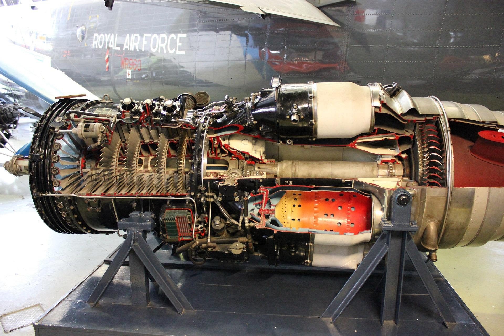
To illustrate how these concepts work together, consider the problem of modeling a turbojet engine. Turbojet operation involves a delicate interplay of air and fuel mass flow, energy conservation, pressure ratios, and non-constant gas properties. Solving for engine performance at any given operating point requires iterative computation across multiple stages, each involving coupled thermodynamic and aerodynamic relationships. Even simplified simulations demand significant computational resources, and full computational fluid dynamics models of even small engine sections can consume tens of thousands of CPU hours.
The specific task chosen for demonstration is autothrottle control: adjusting the throttle to achieve a target change in engine speed at a given altitude while balancing speed-up time against fuel consumption. While classical control methods like gain scheduling have long been used for this purpose and remain easier to certify for safety-critical flight operations, the turbojet problem serves as an excellent testbed for exploring RL and ROM-based transfer learning.
The engine simulation used in this work is based on a high-fidelity Python model, supplemented by a standard atmosphere library that accounts for variations in altitude, temperature, density, and compressibility effects. The aircraft itself is modeled as a hypothetical design scaled from the historical B-47 Stratojet bomber, with aerodynamic parameters including mass, drag coefficient, aspect ratio, wetted surface area, and Oswald efficiency chosen to produce realistic flight behavior.
Aircraft dynamics are discretized at 0.1-second intervals, computing acceleration from the difference between engine thrust and aerodynamic drag at each step. Drag is calculated using standard aerodynamic relationships involving the lift coefficient, which itself depends on the aircraft’s mass, speed, air density, and wing area. The ISA library handles conversions between Mach number, velocity, and altitude throughout the simulation.
## Building the SINDy-Based ROM
To construct a ROM for this system, SINDy requires a dataset of state trajectories paired with their time derivatives. This is generated by running the turbojet simulation across a range of operating conditions — different altitudes, Mach numbers, and throttle settings — and recording the resulting thrust values along with the computed rate of change of velocity.
The SINDy algorithm then searches through a library of candidate terms, including polynomials of throttle setting, to find the simplest equation that reproduces the observed dv/dt behavior. Remarkably, the resulting ROM takes the form of a straightforward cubic polynomial in throttle setting alone:
dv/dt = −3.022 + 1.973 × Throttle − 0.132 × Throttle³
Notably absent from this equation are altitude and Mach number. While this might seem concerning at first glance — after all, both altitude and velocity clearly affect real engine performance — the explanation lies in how the specific simulation and aircraft model were configured. In this particular setup, altitude affects both thrust and drag in compensating ways, and the SINDy algorithm determined that these effects cancel out sufficiently in the training regime to be omitted. The absence of Mach number is more significant, since turbojet thrust is roughly constant with velocity while drag increases, but the practical performance of the transfer learning approach ultimately determines whether this simplification is acceptable.
## Training the RL Agent with Transfer Learning
The reinforcement learning framework uses the Proximal Policy Optimization (PPO) algorithm, a popular and well-regarded method for continuous action spaces. The agent receives as input the current Mach number, altitude, and target Mach number, and outputs a throttle setting between zero and one. The reward signal penalizes fuel consumption, with large negative rewards assigned if the aircraft velocity drops to unphysical levels.
Two separate training runs are compared: a baseline approach where the PPO agent trains directly on the full turbojet simulation, and a transfer learning approach where the agent first trains on the ROM-based environment before being evaluated on the full simulation. The ROM-based gymnasium environment is identical in its state and action spaces to the full simulation version, except that it uses the SINDy-discovered polynomial equation to compute velocity changes and assumes fuel flow scales proportionally with throttle setting.
The performance gains are striking. Training the ROM-based environment for 10,000 timesteps requires roughly 13 seconds, compared to approximately 2,500 seconds for the full simulation to reach 4,000 timesteps. When comparing reward progress at equivalent total elapsed times, the transfer learning agent achieves a reward of −1,170 after about 2,232 seconds of total computing time, while the baseline agent trained directly on the full simulation reaches only −2,080 after 2,596 seconds. In other words, the ROM-based transfer learning approach achieves a substantially better policy in less than half the wall-clock time.
## Broader Implications
The combination of data-driven ROM generation and transfer learning opens up significant possibilities for applying reinforcement learning to complex physical systems that were previously considered computationally intractable. By dramatically reducing the simulation cost per training iteration, ROMs make it feasible to explore RL-based approaches for control, optimization, and analysis of systems ranging from jet engines to power grids to climate models.
Beyond transfer learning for RL, the SINDy methodology itself represents a broader advance in how we model and understand complex physical systems. Data-driven discovery of governing equations can reveal hidden patterns, suggest new simplifying assumptions, and provide compact representations that are useful not only for machine learning but also for classical analysis, design optimization, and real-time control applications.
It is worth noting that the specific implementation described here uses low-order approximations throughout — simple Euler discretization, basic aerodynamic drag models, and a ROM that ignores certain state dependencies. The purpose was not to build a production-grade autothrottle system but to demonstrate the viability of the approach. In practice, higher-fidelity ROMs and more sophisticated RL algorithms would likely yield further improvements.
## Frequently Asked Questions
### What types of physical systems benefit most from ROM-based transfer learning?
Systems with high computational cost per simulation step and large or continuous state spaces benefit the most. Turbomachinery, aerospace vehicles, power systems, and climate models are all natural candidates where traditional simulation is expensive and RL could offer advantages in finding novel operating strategies or robust control policies.
### Why use SINDy specifically for generating ROMs?
SINDy is attractive because it is unsupervised — it does not require prior knowledge of the governing equations or labeled training data. It automatically discovers parsimonious mathematical models from measurement data alone, making it applicable to systems where first-principles models are unavailable, incomplete, or too complex to work with directly.
### Can transfer learning from ROMs degrade the quality of the final policy?
There is always a risk that simplifications in the ROM introduce discrepancies that cause the transferred policy to perform poorly on the full system. Careful validation is essential. In practice, this is mitigated by testing the ROM-trained policy on the full simulation and, if necessary, fine-tuning it further using on-line training with the high-fidelity model.
### How does the ROM training time compare to full simulation training time?
As demonstrated in the case study, ROM training can be orders of magnitude faster. In the example, ROM training took seconds while full simulation training took minutes — and the gap would widen dramatically for more complex simulations where individual time steps take longer to compute.
### Is this approach limited to turbojet engines?
Absolutely not. The methodology is general: generate training data from any dynamical system, apply SINDy or other ROM techniques to discover a simplified model, train an RL agent on the ROM, and transfer the learned policy to the full system. The same framework applies to any physical domain where simulation is costly and data is available.
### What are the limitations of the SINDy approach?
SINDy assumes that the underlying dynamics can be expressed as a sparse combination of candidate basis functions. If the true dynamics involve terms not included in the library, or if the data does not adequately cover the relevant regions of the state space, the discovered model may be incomplete or inaccurate. The quality of the ROM is directly tied to the quality and coverage of the training data.
## Final Thoughts
The marriage of reinforcement learning, transfer learning, and data-driven reduced order modeling represents a powerful new paradigm for tackling complex physical systems. By creating fast, faithful surrogates of expensive simulations, ROMs unlock the practical applicability of RL to domains where training from scratch would be prohibitively slow. The SINDy methodology provides a principled way to construct these surrogates directly from data, even when our theoretical understanding of the underlying physics remains incomplete. As computational datasets grow and machine learning algorithms continue to mature, this combined approach is likely to become an essential tool in the engineer’s and scientist’s toolkit — enabling faster discovery, more robust control, and deeper insight into the nonlinear systems that shape our world.
Thank you for reading
