



# A New Agentic Framework for Automated Quantitative Factor Research and Predictive Modeling
## Introduction
Quantitative finance has long struggled with two distinct but deeply intertwined challenges: discovering meaningful predictive signals (factors) and translating those signals into robust predictive models. Traditionally, both tasks require heavy human intervention — from hypothesizing which relationships might persist in market data to selecting the right model architecture and hyperparameters. A growing body of research is exploring whether AI-driven agent systems can automate these pipelines end to end, reducing human bias and accelerating the pace of discovery.
Recent developments in this space describe a modular, multi-agent framework that tackles both factor discovery and model development in two independent but complementary research loops. The system employs specialized autonomous agents, each assigned a distinct role, and is orchestrated by a central manager that ensures every handoff is traceable and auditable. What follows is an overview of how this architecture works, what it achieves, and why it matters for the future of systematic investing.
—
## The Six-Agent Pipeline for Factor Discovery
The first research loop focuses on generating and validating novel alpha factors. It operates as a six-stage pipeline, with each stage handled by a dedicated agent:
– **Data Steward**: Manages data ingestion, cleaning, and windowing, ensuring that all downstream agents work with consistent, properly formatted inputs.
– **Visual Analyst**: Examines data distributions, identifies anomalies, and surfaces patterns that may warrant deeper investigation.
– **Idea Miner**: Generates falsifiable hypotheses — each specifying a proposed mechanism, a predicted directional relationship, and explicit conditions under which the hypothesis would be refuted.
– **Factor Evaluator**: Constructs candidate factors from a registry of composable time-series and cross-sectional operators, ensuring that every operator works within a well-defined causal boundary (trailing windows for temporal operators, current timestamps for cross-sectional ones).
– **Backtest Engineer**: Runs rigorous out-of-sample backtests, measuring directional accuracy and calibrating factor performance across multiple regimes.
– **Research Librarian**: Maintains a persistent memory store that captures what has been tried, what succeeded, and what failed — feeding this knowledge back into subsequent search cycles.
Crucially, no two agents communicate directly with one another. Every piece of information passes through the central AI Manager, which serves as a single point of coordination. This design choice has a practical benefit: it makes every run fully auditable, since the Manager logs every handoff, decision, and state transition.
### How Factors Are Validated
A factor is never treated as a raw expression to be optimized blindly. Instead, it enters the pipeline as a structured proposal containing:
1. A **hypothesis** — a clear statement about what relationship is expected to exist.
2. A **mechanism** — an economic or statistical rationale for why the relationship might hold.
3. A **predicted direction** — whether the factor should be positively or negatively correlated with future returns.
4. **Refutation conditions** — specific scenarios under which the hypothesis would be considered falsified.
Only after this framing is complete does the Factor Evaluator assemble the factor using standardized operators drawn from a formulaic alpha registry. The resulting factors are then subjected to three nested feedback loops:
– **Direction calibration** within each backtest, ensuring the predicted sign of the relationship holds.
– **Falsification-driven belief updating** within each run, allowing the system to discount hypotheses that fail to meet their refutation conditions.
– **Cross-run memory**, where the Librarian feeds historical results into the Idea Miner, steering future hypothesis generation away from dead ends and toward more promising territory.
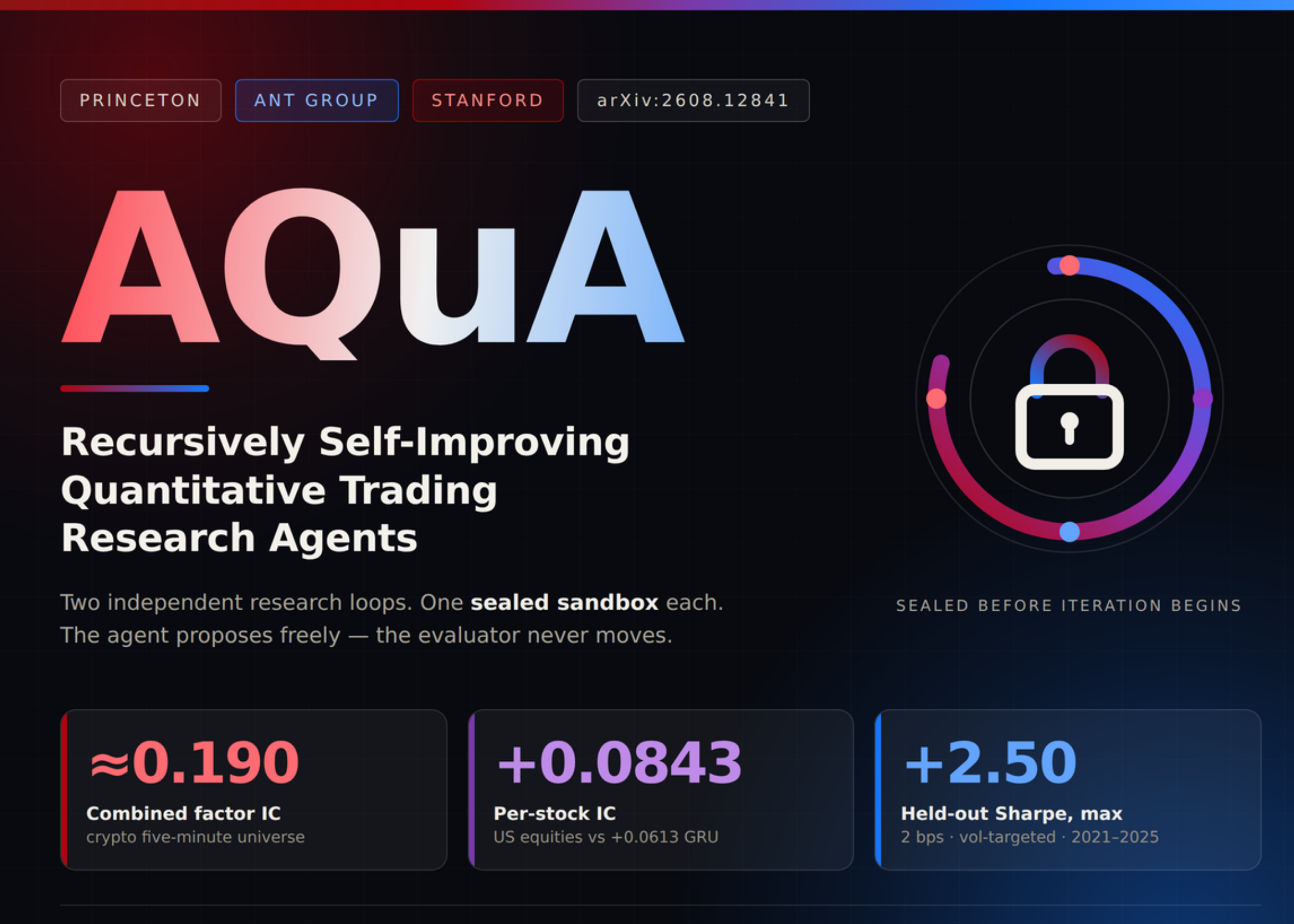
When tested on a cryptocurrency universe with five-minute bars, this pipeline achieved a combined validation Spearman rank correlation (IC) of approximately **0.190** after twenty research epochs. For comparison, adapted versions of prior frameworks produced ICs of 0.171, 0.151, and 0.137, while a standard LSTM baseline reached 0.137 and a LightGBM baseline achieved 0.106. An Alpha158-style baseline scored 0.075.
It is important to note that individual factors generated by the system remain modest — single-factor ICs range from 0.026 to 0.037. The headline performance reflects the power of the *harness* (the pipeline and orchestration framework) rather than any single expression.
—
## Config-Driven Model Development for Intraday Equity Returns
The second research loop shifts focus from factor discovery to predictive modeling. Here, the goal is to forecast each stock’s forward return thirty minutes into the future using intraday US equity data.
### Data Split and Experimental Design
The training protocol is strict and transparent:
– **Training data**: 2010 through 2019.
– **Embargo gap**: 2020 — completely untouched by any part of the pipeline, including feature selection, hyperparameter tuning, or model selection.
– **Test data**: 2021 through 2025 — held out entirely until final evaluation.
Model selection is performed using an inner-validation slice drawn exclusively from the end of the training window. This prevents any form of data leakage from the test period into the model development process.
### Hypothesis-Driven Variant Generation
Each experiment is defined by a single configuration difference — a change in architecture, loss function, sampling strategy, or optimizer. This ensures that every variant produced by the system is comparable against its peers, because all other conditions remain identical.
### The Hybrid Predictor Architecture
The model that emerged as the top performer is a hybrid architecture composed of several stages:
1. **Multi-scale 1-D convolutional front-end**: Extracts patterns across multiple time horizons from raw price and volume feeds.
2. **Configurable backbone**: In the reported run, this was an attention-based module, though the architecture supports LSTMs, Mamba-style state-space models, and transformer attention interchangeably.
3. **Cross-sectional mixing stage**: Integrates information across the entire stock panel at each timestamp, capturing sector and market-wide effects.
4. **Gated fusion**: Combines the temporal and cross-sectional representations using learned gating weights.
5. **Pooled per-stock readout**: Produces a single prediction for each stock in the universe.
### Feature Importance and Model Performance
One of the most striking findings is that no single price or volume feature dominates. The strongest univariate predictor — a simple 5-minute return — carries a correlation of only −0.031 with forward returns, and a ridge regression combination of all standard features reaches merely +0.025. The signal is subtle, diffuse, and distributed across many weak inputs.
Against this backdrop, the model performance on identical data and a shared evaluator is compelling:
| Model | Per-Stock Raw IC |
|——-|—————–|
| Ridge Regression | +0.0251 |
| LightGBM | +0.0397 |
| Extended LSTM | +0.0434 |
| Standard LSTM | +0.0535 |
| GRU | +0.0613 |
| **Hybrid Architecture** | **+0.0843** |
The hybrid model’s IC of +0.0843 represents a **+0.0230 absolute improvement** over the best baseline (GRU), which translates to a **37.5% relative gain**. Notably, the authors emphasize that the IC conventions used in Part I (factor discovery) and Part II (model development) differ and should not be compared directly — each loop has its own validation protocol and metric design.
—
## From Signal to Strategy: Building a Live Trading Book
Having established a predictive signal, the next question is whether it can be converted into a profitable trading strategy. The framework applies the following construction:
– **Portfolio construction**: Per-stock scores are converted into a dollar-neutral, threshold-based long/short book. The round-trip transaction cost is set at two basis points per leg.
– **Sector neutrality**: Positions are neutralized across sectors to isolate the pure alpha signal from sector-level exposures.
– **Volatility targeting**: A causal overlay adjusts position sizes based on predicted volatility, improving risk-adjusted returns.
– **Walk-forward parameter selection**: All parameters — including thresholds, costs, and volatility estimates — are chosen exclusively from past data in a fully causal walk-forward procedure, ensuring no look-ahead bias.
### Results
The final strategy delivers the following performance characteristics:
– **Sector-neutralized Sharpe ratio**: **+2.15** (held-out), with training and held-out values nearly identical — indicating minimal overfitting.
– **Sharpe ratio with causal volatility overlay**: **+2.50**.
– **Sharpe ratio with fully causal walk-forward parameter selection**: **+2.00**.
– **Per-stock R²**: 1.20% — modest but meaningful given the difficulty of intraday prediction.
Year-by-year Sharpe ratios for the held-out period are equally impressive:
| Year | Sharpe Ratio |
|——|————-|
| 2021 | +1.7 |
| 2022 | +3.5 |
| 2023 | +1.9 |
| 2024 | +1.8 |
| 2025 | +2.7 |
Every single year posts a positive Sharpe ratio, including the turbulent 2022 period — a period when many quantitative strategies experienced severe drawdowns. This consistency across market regimes speaks to the robustness of the underlying signal and the care taken in the validation protocol.
—
## Key Takeaways
1. **Two independent research loops**: Factor discovery and model development share no agents, memory, or state — reducing contamination between the two tasks and enabling each to be evaluated on its own merits.
2. **Asymmetric freedom**: Agents are free to explore within a well-defined domain-specific language (DSL), but the split of data, feature engineering, label construction, and the evaluator are sealed — preventing the system from inadvertently overfitting to its own methodology.
3. **Strong combined performance**: The factor discovery loop reaches a combined IC of approximately 0.190 on crypto, while the model development loop achieves a per-stock IC of +0.0843 on equities — a 37.5% relative improvement over the best standalone model baseline.
4. **Robust live strategy**: The equity strategy holds a Sharpe ratio of +2.50 at a cost of two basisps and is positive in all five out-of-sample years from 2021 through 2025.
5. **Auditability by design**: The centralized manager architecture ensures that every decision point in the pipeline is logged and traceable, addressing one of the key criticism of automated ML systems in finance.
—
## Frequently Asked Questions (FAQ)
### Q1: What makes this framework different from standard automated machine learning (AutoML)?
Standard AutoML systems typically optimize a single pipeline end to end — selecting features, choosing a model, and tuning hyperparameters simultaneously. This framework separates concerns by running two entirely independent loops (factor discovery and model development) with no shared state, agents, or memory. Additionally, it enforces a strict hypothesis-testing discipline: every factor must be falsifiable before it enters the pipeline, and every model variant is defined by exactly one configuration change, ensuring clean comparisons.
### Q2: Why are individual factor ICs so low if the combined pipeline IC is high?
The combined IC of approximately 0.190 reflects the aggregated output of many factors working in concert, not the strength of any single factor. Individual factors score between 0.026 and 0.037 IC — each is a weak signal on its own. The value lies in the *harness*: the ability to generate, test, and combine many weak signals into a coherent whole, rather than relying on one strong but potentially fragile expression.
### Q3: How does the system prevent overfitting given the complexity of the two-loop architecture?
Several mechanisms work in tandem:
– The embargo gap (2020) ensures that nothing in the training process sees the test period.
– Inner validation is restricted to the end of the training window only.
– The hypothesis-driven structure forces each factor to specify refutation conditions *before* it is tested.
– The walk-forward protocol ensures that no parameter is ever chosen using future data.
– The two research loops are entirely independent, so overfitting in one loop cannot leak into the other.
### Q4: What is the significance of the 2-basis-point transaction cost assumption?
Two basis points per leg (four basis points round-trip) represents a realistic estimate for liquid US equities when accounting for bid-ask spreads and market impact. The fact that the strategy maintains a Sharpe ratio above +2.00 even after deducting these costs suggests that the signal has genuine economic value and is not an artifact of assuming frictionless trading.
### Q5: Why does the paper emphasize that the Part I and Part II ICs should not be compared?
The two loops use different validation protocols, different data universes (crypto five-minute bars versus intraday US equities), and different metric conventions. Part I measures combined Spearman IC across 20 research epochs on a crypto universe, while Part II reports per-stock raw IC on a held-out equity test set from 2021–2025. Comparing them directly would be misleading, as they answer fundamentally different questions.
### Q6: Can this framework be applied to other asset classes or timeframes?
The architecture is intentionally general. The DSL-based operator registry, the modular agent pipeline, and the config-driven model development loop are all designed to be swapped across domains. The framework has been demonstrated on crypto and intraday equities, but the same principles — falsifiable hypotheses, causal operator composition, strict out-of-sample validation, and centralized auditability — could be applied to foreign exchange, fixed income, commodities, or longer-horizon data with appropriate adjustments.
—
## Conclusion
The convergence of agentic AI systems and quantitative finance represents a significant step forward in how alpha is discovered and deployed. By decomposing the research process into specialized, auditable roles and enforcing rigorous validation discipline at every stage, this framework offers a compelling template for systematic factor research and model development.
The results speak for themselves: a combined factor IC of 0.190 on crypto, a per-stock predictive IC of +0.0843 on equities that outperforms the best baseline by 37.5%, and a live trading strategy delivering a Sharpe ratio above +2.50 across five consecutive years — including a year defined by market stress and drawdowns.
What is perhaps most encouraging is the philosophy underlying the work: that automation and rigor are not at odds. By making every hypothesis falsifiable, every handoff auditable, and every parameter choice causal, the system achieves both flexibility and discipline. As quantitative research becomes increasingly complex and data-rich, frameworks like this one point toward a future where AI agents serve not as black-box oracle machines, but as transparent, accountable research partners that augment human insight rather than replace it.
—
Thank you for reading
