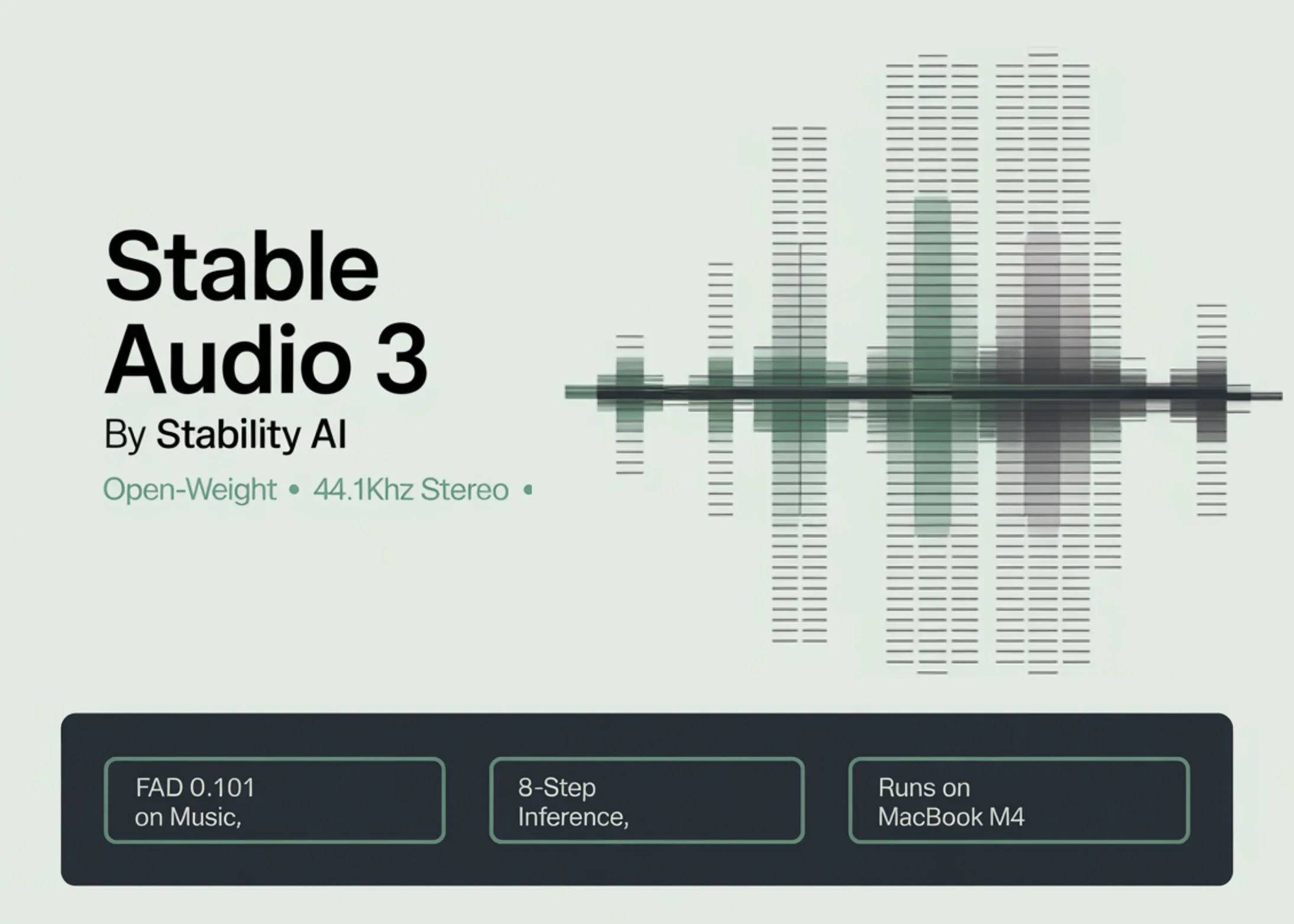
Stability AI Unveils Stable Audio 3: Next-Gen Latent Diffusion Models for Lightning-Fast Audio Creation and Editing

Stability AI has made the open weights for Stable Audio 3 publicly available, along with a detailed technical research paper. Stable Audio 3 is a collection of latent diffusion models designed to produce stereo audio at a 44.1 kHz sample rate. These models offer support for variable-length audio generation, editing through inpainting, and rapid inference speeds.

What Is Stable Audio 3?

Stable Audio 3 comes in three different model sizes: small, medium, and large. At its core, a latent diffusion model works by learning to gradually strip away noise from a compressed version of audio, known as a latent. Through training on numerous pairs of noisy latents and their corresponding clean audio, the model learns how to transform random noise into coherent audio.

The three model sizes vary in their capacity and the maximum length of audio they can generate. All parameter counts listed below refer specifically to the diffusion transformer component. Each model also incorporates a SAME autoencoder (with 108 million parameters for SAME-S and 852 million for SAME-L).

• small-music — 459 million diffusion transformer parameters, capable of generating up to 2 minutes of music-only content.
• small-sfx — 459 million diffusion transformer parameters, capable of generating up to 2 minutes of sound effects only.
• medium — 1.4 billion diffusion transformer parameters, capable of generating up to 6 minutes and 20 seconds of both music and sound effects.
• large — 2.7 billion diffusion transformer parameters, capable of generating up to 6 minutes and 20 seconds of both music and sound effects.

The small and medium model weights are openly accessible on Hugging Face. The large model is available under an enterprise license.

Architecture: Two Components

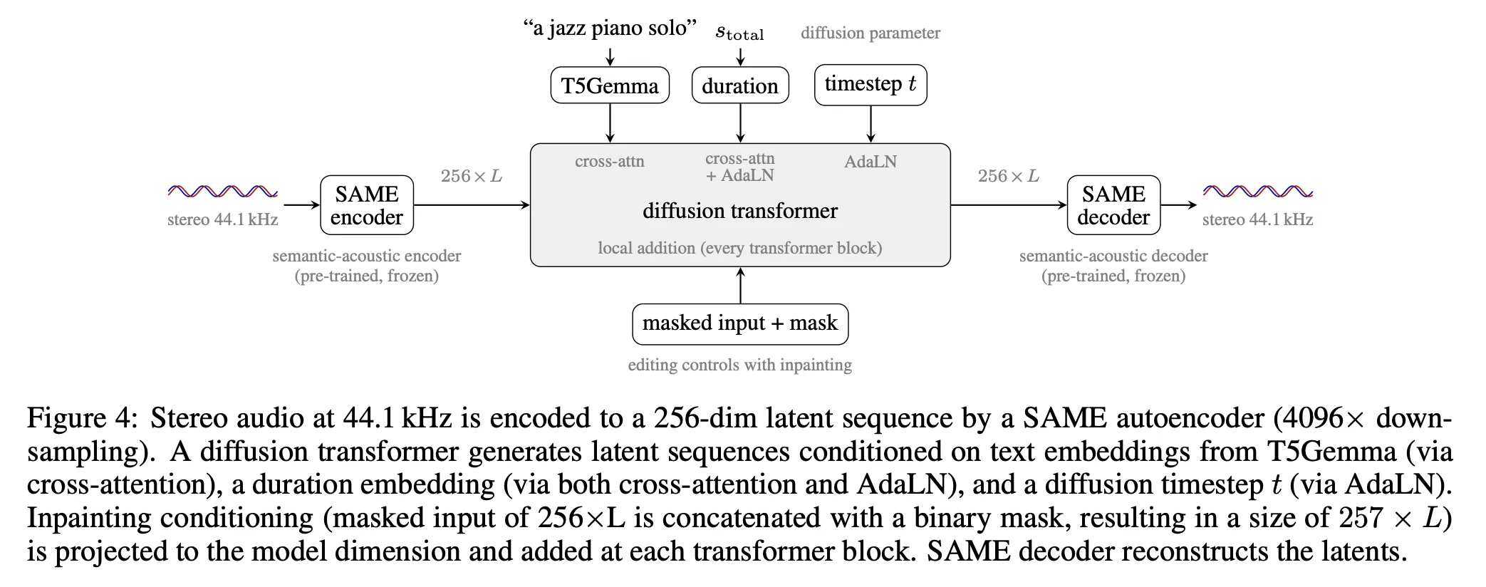
Stable Audio 3 is built around two primary components: a semantic-acoustic autoencoder named SAME, and a diffusion transformer responsible for generating latent sequences based on text prompts, desired duration, and inpainting masks.

The SAME Autoencoder

SAME (Semantically-Aligned Music autoEncoder) transforms stereo 44.1 kHz audio into a compact latent representation and reconstructs it back. Its standout design feature is a 4096× downsampling ratio — significantly greater than the 1024× to 2048× ratios typically found in earlier audio autoencoders. This elevated ratio shortens latent sequences sufficiently to make long-form audio generation feasible on consumer-grade hardware.

SAME accomplishes its 4096× compression in two phases. The first is a patching stage, which reorganizes stereo audio into non-overlapping segments of 256 samples per channel, achieving 256× downsampling. The second phase uses a Transformer Resampling Block (TRB), which applies an additional 16× downsampling through learnable output embeddings woven into the input sequence and processed by a transformer. The result is a 256-dimensional latent sequence running at roughly 10.76 Hz for a 44.1 kHz input.

The SAME autoencoder is trained using five distinct loss functions: spectral reconstruction, adversarial, diffusion alignment, semantic regression (which predicts chroma and interaural level difference), and contrastive latent alignment. Together, these losses ensure the latent representation maintains both high-quality acoustic reconstruction and meaningful semantic structure. A soft-normalisation bottleneck keeps the latent values within a defined range, enabling deterministic encoding.

Once trained, the SAME autoencoder remains frozen during diffusion training. The small models use SAME-S (108 million parameters, optimized for CPU-based inference), while the medium and large models use SAME-L (852 million parameters).

The Diffusion Transformer

The Diffusion Transformer processes latents of the SAME size. External conditioning is delivered through three separate channels:

1. Text conditioning — a pre-trained, non-trainable T5Gemma encoder generates 256 embedding vectors of 768 dimensions. For shorter text inputs, padding is handled with a dedicated learnable embedding to fill up to the 256-token limit; longer inputs are simply cut off.
2. Duration conditioning — duration information is transformed into a Fourier features vector and then fed into the system using two methods: Adaptive Layer Normalization (AdaLN) and cross-attention, both merged with the text prompt representation.
3. Inpainting conditioning — a binary mask (marking which portions to fill in) combined with the pre-masked reference audio is passed through a compact 2-layer MLP, and the resulting signal is injected into the residual stream within every transformer block.

Every transformer block is composed of the following elements: self-attention, cross-attention, local-additive conditioning specific to inpainting, and a SwiGLU-based feed-forward network. Both the medium and large model variants use differential attention — a technique where two independent attention maps are computed from two separate (Q, K) head pairs that share a single V, after which the second map is subtracted from the first. This effectively suppresses patterns that are common between the two heads, amplifying more meaningful distinctions. The transformer also appends 64 learnable memory embeddings at the front of every sequence before any processing begins. These act as a shared global context buffer that any position in the sequence can reference. They are stripped out before any loss calculation is performed.

Variable-Length Generation

Most existing latent diffusion models for audio are restricted to a fixed maximum sequence length. When you produce a short clip, the entire computation runs at the full preset length, wasting resources on blank, silent frames. Stable Audio 3 is natively trained to handle variable-length outputs using three complementary techniques:

• Variable-length flash attention combined with masked loss — sequences shorter than the longest one in a batch are padded on the right in latent space. Padded positions are excluded from self-attention calculations and do not contribute to the loss.
• Per-element timestep adjustments — because longer sequences contain more redundancy between adjacent elements, they tend to preserve more structure at the same noise level. To account for this, during training the noise schedule is shifted toward higher noise values for longer sequences. This is done using a logistic shift controlled by the parameter μ, which interpolates between μ_min=0.5 and μ_max=1.15 depending on the sequence’s length.
• Silence augmentation — the real audio segment is randomly extended with pre-computed silence embeddings sampled from an exponential distribution, on average adding 4 seconds. This teaches the model to wrap up audio with smooth, natural-sounding silence.

The end result is that inference cost directly reflects how long the output is. The medium model can render 20 seconds of audio in roughly 0.62 seconds on an H200 GPU. Producing 380 seconds of audio on that same hardware takes 1.31 seconds.

Three-Stage Training Pipeline

Stage 1 — Flow Matching Pre-Training. The model is trained to learn a velocity field that gradually transforms Gaussian noise into audio-compatible latent representations. The training objective uses minibatch optimal transport coupling, implemented via Sinkhorn iterations. This method pairs each ground-truth data sample with the closest noise vector available within the current mini-batch, resulting in straighter training trajectories and fewer intersecting transport paths. Inpainting is integrated throughout training from the start: at each training step, one of three mask strategies is randomly chosen — a full mask (80% chance, corresponding to unconditional generation), randomly placed segment masks (10% chance), or a causal prefix mask used for audio continuation tasks (10% chance).

Stage 2 — Distillation Warmup. A frozen copy of the flow matching model now serves as the teacher, producing full 15-step DPM++ trajectories using classifier-free guidance (CFG) at scale 5. The student model is trained for 10,000 steps with the task of mapping any noisy intermediate state directly to the teacher’s final denoised output — a single step. The loss function is mean squared error (MSE). This effectively collapses what was a multi-step ODE into a single-step denoising operation. The downside is that MSE averaging pushes predictions toward the conditional mean, which tends to dull fine details.

Stage 3 — Adversarial Post-Training. This phase moves past the MSE objective entirely and instead employs a relativistic adversarial training framework. A discriminator — built from the original flow matching model’s weights — directly evaluates the student’s one-step denoised outputs against genuine data. The teacher model from Stage 2 is no longer needed and is fully discarded. The generator is optimized using two losses: a relativistic adversarial loss (L_R) and a CLAP alignment loss (L_CLAP). The discriminator itself is optimized with L_R along with a contrastive loss (L_C) that penalizes it whenever it fails to account for text-audio correspondence — it learns to correctly distinguish authentic audio-text pairings from randomly shuffled ones. This adversarial approach lets the model restore the perceptual sharpness that was lost during MSE distillation.

Inference: Ping-Pong Sampling and No CFG

After adversarial training, the model is capable of producing audio in a single forward pass. In practice, generating from pure noise in one step is still challenging, so Stable Audio 3 introduces ping-pong sampling at inference time. In this approach, the model first denoises the signal until a clean estimate is reached, then re-adds a controlled amount of noise at a lower intensity, and then denoises again. This repeat-denoise-then-renoise cycle runs for 8 iterations on a logSNR-uniform schedule — that is, N+1 evenly spaced steps spanning the range [λ_min, λ_max] = [−6.2, 2.0]. Each new iteration has the chance to fix imperfections introduced in the previous one.

A notable design choice: Stable Audio 3 does not use classifier-free guidance (CFG) during inference. Conventional diffusion models run two forward passes at every sampling step — one conditioned on the prompt and one unconditionally — then blend the two. In Stable Audio 3, the quality improvements normally gained from CFG are folded into the model during Stage 2, where the student learns to match teacher trajectories that were themselves generated with CFG. Text-audio alignment is further tightened through the CLAP loss (L_CLAP) during Stage 3. That means the extra computational cost of CFG at inference — doubling the number of model passes — is completely eliminated.

Prompt formatting requirement: All Stable Audio 3 model variants — small-music, medium, and large — which were trained on the AudioSparx dataset prompt prefixes to work as intended. For music, prompts should begin with the prefix "TrackType: Music, VocalType: Instrumental,". For sound effect prompts, begin with "TrackType: SFX,".

Evaluation Results

Instrumental music (Song Describer Dataset, 120s clips). On the FAD metric (where lower scores are better) and CLAP scores (where higher is better), the large model scores FAD 0.101 / CLAP 0.393. The medium model achieves FAD 0.107 / CLAP 0.390. For comparison, Stable Audio 2.5 — the internal previous-generation baseline — achieves FAD 0.106 / CLAP 0.395. In human listening evaluations, both medium and large outperform Stable Audio 2.5 on musicality (MUS): medium and large score 4.15 and 4.30 respectively out of 5, versus 3.70 for Stable Audio 2.5. Generating a 120-second audio clip on an H200 takes 0.45s with the small model, 0.78s with medium, and 0.81s with large. Stable Audio 2.5 requires 0.85s for the same duration.

Sound effects (BBC Sound Effects Dataset, 5s clips). The medium model achieves FAD 0.369 / CLAP 0.369. The strongest competing open-weight baselines are Stable Audio Open Small (FAD 0.500 / CLAP 0.277) and Stable Audio Open (FAD 0.501 / CLAP 0.263). Woosh Flow trails behind with an FAD of 0.580.

Audio editing via inpainting. The researchers assess inpainting performance across three categories:

settings: single region, two independent regions, and continuation. For music, medium achieves FAD-full of 0.046 on single inpainting and 0.046 on double inpainting. Large achieves 0.047 on both. For continuation, medium achieves FAD-full 0.074 and large achieves 0.071. Sound effects results follow a similar pattern; continuation shows higher FAD than inpainting in both domains, which the team attributes to the model having less surrounding audio context to anchor the generation.

Comparison

Key Takeaways

• Stable Audio 3 is a family of open-weight latent diffusion models (small, medium, large) for music and sound effects generation and editing.
• A SAME autoencoder with 4096× downsampling compresses audio into 256-dimensional latents at ~10.76 Hz, making long-form generation tractable on consumer hardware.
• Variable-length generation is natively supported: inference cost scales with requested duration, not a fixed maximum length.
• Three-stage training (flow matching → distillation warmup → adversarial post-training) enables 8-step inference without classifier-free guidance.
• Prompt prefixes ("TrackType: Music, VocalType: Instrumental," / "TrackType: SFX,") are required for AudioSparx-trained model variants.

Check out the Paper, Model Weights and Repo here. Also, feel free to follow us on Twitter and don’t forget to join our 150k+ ML SubReddit and subscribe to our Newsletter. Wait! Are you on Telegram? Now you can join us on Telegram as well.

Need to partner with us for promoting your GitHub repo, Hugging Face page, product release, webinar, or more? Connect with us.